13.3: The Universe is Expanding

Learning Objectives

• You will know that the Hubble law is evidence that the Universe is expanding.
• You will know that the Universe is expanding, but individual galaxies are not.
• You will know that there is no center or edge of the Universe.

Expansion or Explosion?

Interpretation of the Hubble Law

The observation of galactic redshifts from the 1920s and thereafter was the main motivation for the Big Bang theory. It is very difficult to explain these observations in terms of independent motions of galaxies through space. After all, the galaxies are billions of light-years away from each other. How could they all conspire to move in the same way? Many people, when they hear the term ‘Big Bang,’ imagine some sort of explosion, like a giant firecracker, but that is problematic because it is not consistent with a number of observed properties of the Universe. The actual Big Bang theory is something quite different. From the perspective of general relativity it is much more natural to explain the redshift-distance relation in terms of galaxies that are embedded in a space that is uniformly expanding.

If we abandon the scenario in which galaxies are moving through space, we are left with one where space itself expands and carries galaxies along as it does so. General relativity provides a context in which the notion of expanding space makes sense. In fact, if general relativity is an accurate theory of the behavior of space and time, it is very difficult to contrive a situation in which the Universe could be static. Given the success of general relativity in explaining many individual phenomena (gravitational lenses, precession of orbits, etc.), it is natural to think of space overall as either expanding or contracting.

Even in a Newtonian analog the idea of a static Universe is difficult to make work: think how surprised you would be to see a ball simply hovering some distance above Earth’s surface. If you looked at a photograph showing a ball in that position, you would assume that it must be either rising or falling. An analogous scenario is true for the Universe on grander scales: when we look at any given galaxy we are essentially seeing a snapshot of it. General relativity provides a framework for understanding how that snapshot relates to the ongoing evolution of the Universe.

It is worth elaborating on how an expanding space differs from a static space with objects moving through it. Without general relativity, we are not used to thinking of space as having properties of its own, so we will use several analogies.

One way to imagine space is like a stretchy band with galaxies stuck onto it (Animated Figure 13.5). As the band stretches, the galaxies all move away from each other, but they are moving due to the stretching of the space, they are not moving through the space. Furthermore, we see that the galaxies themselves are not stretching, they are not growing, only the space between them is. That is because the internal (gravitational) forces within galaxies overwhelm the expansion. So our Universe is expanding, but our Galaxy and Solar System are not. On average, all galaxies are moving away from each other, but within a galaxy, the stars are not moving away from each other because gravity keeps them bound together.

Animated Figure 13.5: An analogy for the expansion of space: a stretchy band. The galaxies move away from each other as space stretches. They never actually move along the band; they are just along for the ride. The galaxies themselves do not expand, only the space between them. Credit: NASA/SSU

Continuing with this analogy, we can explain the Hubble Law: galaxies are getting farther apart from each other more quickly the farther apart they are from each other. Figure 13.6 illustrates this principle in one dimension. We can imagine that the galaxies (A, B, C, D) are on the band in a line and are a certain distance apart (say 1 cm) at a given moment. The band then expands such that all of the galaxies will be 1 cm farther apart from adjacent galaxies at some time (say 1 second) later.

In this scenario, not only will the galaxies be farther apart than before, but the farther apart they started from each other, the more they will have been carried along with the expansion. From the perspective of galaxy A, galaxy B started off 1 cm away and is 2 cm away 1 second later. So from A’s perspective, B moved away at 1 cm/s. Similarly, galaxy C started 2 cm away from A and is 4 cm away 1 second later. It moved the distance between A and B plus the distance between B and C, or a total distance of 2 cm. That means C moved away from A at 2 cm/s. Galaxy D started off 3 cm away from A and moved away at 3 cm/s. This follows a linear relationship. If we plotted the distances of the points A, B, C and D vs. their motions, we would get a line, just like in a Hubble diagram.

It does not matter which point you choose as a reference in this exercise. You will always get the same linear expansion law. From the perspective of Galaxy B, for example, galaxy A was 1 cm away and moved away at 1 cm/s. Galaxy C was also 1 cm away from B and moved away at 1 cm/s due to the expansion of the band. Galaxy D was 2 cm away and moved away from B at 2 cm/s.

Again, an important thing to realize is that none of these galaxies exerted any effort to move. They were carried along with the expansion, or stretching, of the fabric of space. For simplicity we have done this example in one dimension (a line), but this sort of stretching happens in all three spatial dimensions simultaneously as the Universe expands.

Figure 13.6: An analogy for the expansion of space: a stretchy band. The galaxies move away from each other as space stretches. The expansion follows the Hubble Law: the farther away a galaxy is from another, the faster its velocity. This is true from the perspective of any of the galaxies. Only one dimension is shown here but the fabric of space stretches in all three spatial dimensions as the Universe expands. Credit: NASA/SSU/Aurore Simonnet

In addition to being carried along with the expansion of space on the largest scales, galaxies are also moving in ways not due to the expansion of the Universe. These motions, known as peculiar velocities, are caused by local conditions near the galaxies, for example the tug of gravity from galactic neighbors. An analogy for this would be to imagine ants crawling around on an expanding picnic blanket. The crawling around motions of the ants would be analogous to the peculiar velocities of galaxies. On average, all of the ants would be getting farther away from all of the other ants because of the expansion of the blanket, just as all galaxies on average are getting farther away from all other galaxies due to the expansion of the Universe. Any particular ant would see its closest neighbors moving in many different directions, even after the blanket has begun to stretch.

For nearby ants, the peculiar motions are greater than the very slow stretching separation between them. In contrast, each ant sees the most distant ants moving rapidly away from itself due to the accumulated stretching of the blanket that is occurring between them. The peculiar motions within a distant group become comparatively unimportant and are even undetectable between groups with large separations. This illustrates what is meant by saying that space is expanding and carrying objects along with it, in contrast with saying the objects are moving through space.

One final analogy may help you visualize why we say the Universe expands (space stretches) but galaxies do not. Imagine making a loaf of raisin bread (Figure 13.7). Before baking, the raisins are scattered around in the dough. Each raisin would be stuck in a particular position within the loaf of bread dough. As the bread bakes and rises, the volume of bread increases. And as in our other analogies, two raisins will see their distance from each other increase even though they have not moved “through” the dough (i.e. the "space"). Instead, they have been carried along by the expansion of the dough.

An important feature of the expansion of the Universe is that the galaxies themselves do not expand, only the space between them does. In the raisin bread analogy, the dough rises but the raisins stay the same size. In the Universe, the internal forces in galaxies, stars, people, and other objects overwhelm the expansion locally, so they remain the same size/distance while the expansion of space carries them farther away from one another on large scales.

Figure 13.7: Another analogy for the expansion of space is a loaf of raisin bread baking; the raisins are like galaxies and the dough is like space. Credit: NASA/SSU/Aurore Simonnet

Each of these analogies is meant to help you visualize the three-dimensional stretching of space that takes place as the Universe expands. There is a major limitation shared by all of these analogies that we should mention: each of them features something expanding into space. In the actual Universe, space itself is expanding. It is not necessarily expanding into anything. So, for example, the Universe does not necessarily expand into previously existing empty space. The expansion is instead caused by creation of new space everywhere, constantly.

In the next activity, you will explore the Hubble Law and its implications for the expansion, or stretching, of space.

The Stretching of Space

In this activity, you will see representations of a set of galaxies in the Universe at different times. Between each time the Universe will stretch. You will be able to explore this expansion from the viewpoint of several different galaxies.

To view the Universe from a particular galaxy’s viewpoint, place the red circle over that galaxy.

Play Activity

A. Imagine you are an inhabitant of galaxy A

B. Now imagine you are an inhabitant of galaxy B

C. Center of the Universe

We have just seen that a homogeneous Universe that stretches according to a Hubble Law remains homogeneous. This means the stretching looks the same (on average) at every location. This property, homogeneity, does not hold for other possible explanations for the Hubble Law. The next activity gives an illustration of how homogeneity can be broken under one particular expansion scenario.

The stretching Universe also appears the same (on average) in all directions. We call this property isotropy, and we say that the Universe is isotropic. If you think about it you can probably convince yourself the homogeneity implies isotropy, but not the converse.

Consider the “ancient explosion” scenario that many students initially picture when thinking about how the Universe formed. If all of the galaxies we see are moving away from our location because of some ancient explosion, we should see a different pattern of recession velocities, as well as other consequences of the explosive event. For instance, we might expect that the density of galaxies would be higher toward the center of the explosion, while it would be lower far from the center. We thus would expect to see, at the very least, a difference in density of galaxies in different directions. We do not. In fact, one of the basic observational constraints we have is that the Universe appears the same (on average) in all directions—in other words, that the Universe is isotropic. Another basic observational constraint we have is that the average density of galaxies on large scales is constant (in space, not in time) everywhere—in other words, the Universe is homogeneous on large scales. Obviously, on small scales the density is not constant, but on scales much larger than galaxy clusters it is.

The fact that we observe the Universe to be both homogeneous and isotropic makes it essentially impossible to reconcile the Hubble Law with an explosion of matter out from a single point in space. We certainly would not see an isotropic pattern of galaxies on the sky unless we happened to be at the very center of the explosion. Even then, we would not expect to see the homogeneity that is observed. A better explanation, one consistent with the properties we see in the Universe, is that space is expanding, or stretching.

Explosion Cannot Explain the Observations

As you move the slider bar, you will see representations of a set of galaxies in the Universe at different times. This time there has been a central explosion that shoots matter outward.

Play Activity

General Relativity and the Expansion

If we wish to describe the space of the Universe using general relativity, we know that we will have to write down a spacetime interval that describes the separation between events in that space. But what would such a space look like? It would have to be homogeneous and isotropic, and it would have to expand (or contract) in time. The spacetime interval (\(s^2\)) for such a space (ignoring curvature for now), would look like the expression below.

\[s^2=S^2(t)(Δd)^2−(cΔt)^2\nonumber \]

where \(s^2\) is the interval, \(\Delta d\) is the spatial component, \(c\Delta t\) is the time component, and \(S(t)\) is a stretching factor called the scale factor. We use parentheses with \(S(t)\) to emphasize that the scale factor is a function of time. The purely spatial part of the interval, \((\Delta d)^2\) is defined as follows.

\[(Δd)^2=(Δx)^2+(Δy)^2+(Δz)^2\nonumber \]

The expression should look familiar from the Pythagorean theorem.

This spacetime interval looks exactly like the one for special relativity except that it has the extra term \(S(t)\), the scale factor. The scale factor is a function that describes how space stretches (or contracts) with time. When the spacetime interval is written this way, the scale factor affects all directions equally. Therefore, since normal three-dimensional space is already homogeneous and isotropic, this spacetime interval will be as well.

This is a general form for a spacetime interval that describes a homogenous space which is not curved. We do not need to scale time since it is space that is homogenous and isotropic, not space and time. When we refer to a homogenous and isotropic spacetime we mean that only the space parts are homogenous and isotropic; the Universe is not the same in the past as in the present and in the future.

We still have not put any curvature into this equation, i.e. there are no curvature terms present. The equation describes a flat Universe, one that is not curved in any direction. The term “flat” may conjure up images for you of space being only two dimensional, but notice that we have included all three dimensions in our equation. In the context of cosmology and geometry, “flat” is a technical term and it simply means a lack of curvature.

To understand why our equation does not cause space to curve, we will examine what happens before and after space is stretched. Combining our equations, we have an overall expression:

\[s^2=S^2(t)[(Δx)^2+(Δy)^2+(Δz)^2]−(cΔt)^2\nonumber \]

Consider a particular time, t_o. At that time the scale factor has a value that we could call \(S_0 \equiv S(t_0)\). Plugging into the above equation, the spacetime interval is given by:

\[s^2=[(S_0Δx)^2+(S_0Δy)^2+(S_0Δz)^2]−(cΔt)^2\nonumber \]

We have definitely stretched the space, since our coordinates all have new values now: \(x\) has become \(S_0 x\), \(y\) has become \(S_0 y\) and \(z\) has become \(S_0 z\). \(S_0\) is the same number in all three cases. However, since we have stretched each direction by the same amount (the number \(S_0\)) everywhere, the space remains flat, i.e. it does not curve.

Since there is no curvature in the evenly-stretching interval we have written above, there is not any gravity either. We will add gravity later by ensuring that the interval satisfies Einstein’s field equations. For the moment we are only considering how to describe a homogeneous, isotropic and expanding spacetime.

Describing an Expanding Universe: Comoving Coordinates

In order to more easily discuss the relationships among objects in a dynamic space that can be expanding or contracting, we introduce the concept of comoving coordinates. The core idea of comoving coordinates is to have a system to distinguish between an object moving through space versus an object sitting still in space while being carried away from other objects because space itself is expanding. Comoving coordinates remain fixed for an object as long as it does not move around through space.

We could draw such coordinates on a rubber sheet and then stretch the rubber sheet—the coordinates would remain fixed, but vertices on the sheet would move apart as the sheet itself expanded. Even though the physical distance between two points on the sheet would increase as the sheet stretched, the comoving distance (the coordinates of any point) would be unchanged. This is because the marks would still be in the same spots on the sheet, but additional space (surface area in this example) would be created between them.

Using comoving coordinates, it is easy to represent expansion or contraction in a uniform space. If you place a collection of stationary objects at different points in space, they will stay at the same comoving distance from each other no matter what the space does. The physical distance between them does change, however. This change can be related to their comoving distances with just a single parameter, the scale factor, S, introduced in the last section. This formulation suggests a convenient way to compare different times in the history of the Universe.

We do not know the absolute size of the Universe, and indeed it may be infinite. For this reason it is more convenient to consider the size history of the Universe in relative terms. We can define a scale factor such that \(S=1\) today and \(S=0\) at the moment that the Universe (the existence of space and time) began. With this definition, the physical distance \(d(t)_{physical}\) between two objects at any time \(t\) is just their (unchanging) comoving distance \(d(t)_{comoving}\) multiplied by the scale factor at that time \(S(t)\).

\[d(t)_{physical}=d_{comoving}S(t)\nonumber \]

In Figure 13.8, the “Universe” has expanded by a factor of two from the first panel to the second panel and by another factor of two from the second panel to the third panel. The physical distance between the two points shown depends only on the scale factor at the particular time of the measurement since the comoving distance between them does not change. Only S changes with time; the positions of objects in the comoving system do not.

Figure 13.8 As a rubber sheet stretches, a coordinate grid drawn on its surface will also expand, carrying adjacent vertices away from each other as the surface area of the sheet increases. The grid blocks are comoving coordinates, which remain the same even as the space expands. The purple lines are lines of constant physical size. If the orange lines are measured in comoving coordinates, their lengths are always 1. However, their physical sizes grow, so their lengths become larger relative to the purple lines. Credit: NASA/SSU/Aurore Simonnet

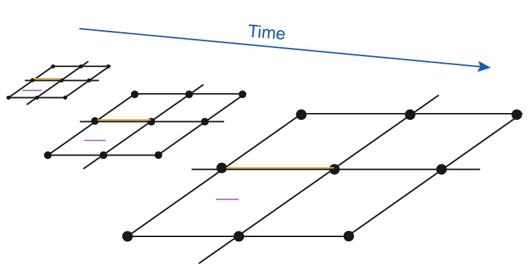
We generally pick the reference time at which we set \(S=1\) to be the present time. This is just for convenience. Then the comoving coordinates are the same as the physical coordinates at the present time. We can find the physical coordinates at other times by multiplying the current physical coordinates by \(S(t)\) for the suitable value of the time, \(t\).

In the next two activities, you will explore the relationship between physical distances, comoving coordinates, and the scale factor.

Comoving Coordinates

In this activity, you will be able to adjust the scale factor for the Universe, measure physical distances, and measure comoving coordinates. Galaxies will be represented by different color dots in this activity.

• To adjust the scale factor, move the slider bar. A scale factor of 1 is the present, a scale factor of less than 1 is the past, and a scale factor of more than 1 is the future.
• To measure the comoving distance between two galaxies, count the number of grid blocks between them.
• To measure the physical distance between two galaxies, check the measure button, then click and drag the line between the two galaxies.

Play Activity

Find two galaxies that are 4 grid spaces apart. Call these galaxies A and B. (You may need to reload the activity if you don’t see two galaxies that fit this criterion at first.)

A. The Present.

Set the scale factor to 1.0.

B. The Past.

Set the scale factor to 0.5.

Using the Scale Factor

Worked Example

1. Galaxies A and B are 50 Mpc apart today, when the scale factor is 1. This is their physical separation.

a. What is their comoving distance today?

• Given: d_physical = 50 Mpc, S = 1
• Find: d_comoving
• Concept: d(t)_physical = d(t)_comoving S(t)
• Solution: 50 Mpc = (d_comoving)(1) → d_comoving = 50 Mpc

b. What was their comoving distance apart at a time in the past when the scale factor was 0.5?

By definition, the comoving distance is always the same. In this case, it is 50 Mpc.

c. What was their physical distance apart at a time in the past when the scale factor was 0.5?

• Given: d_comoving = 50 Mpc, S = 1
• Find: d_physical
• Concept: d(t)_physical = d(t)_comoving S(t)
• Solution: d_physical = (50 Mpc)(0.5) → d_physical = 25 Mpc

So, when the scale factor was half of what it is today, the physical separation between galaxies A and B was half of what it is today. However, the comoving distance is the same today and in the past.

You may have noticed from the previous activity that if a pair of objects are being separated by Hubble expansion, the ratio of their physical distance in the past to their physical distance today is equal to the ratio of the scale factor in the past to the scale factor today. This holds true for the future as well. Mathematically, this can be expressed as below.

\[\frac{d(t_1)_{physical}}{ d(t_2)_{physical}}=\frac{S(t_1)}{S(t_2)}\nonumber \]

where \(t_1\) and \(t_2\) are any two times in the past, present, or future of the Universe.

The Cosmological Redshift

When Edwin Hubble noticed that all galaxies were redshifted, he interpreted that observation as meaning that they were Doppler shifted, and that they moved away from him through space. We stated earlier that the redshift is actually correctly interpreted as being due to the expansion of space. With the spacetime interval for a homogenous and isotropic spacetime and the idea of comoving coordinates we are now ready to explore this idea further: these give us a notion of space itself stretching and carrying objects along with it. This cosmic stretching has a profound effect on light.

When we look at the spectrum of an astronomical object, the redshift, \(z\), is defined as the wavelength shift in some spectral feature, divided by the unshifted wavelength.

\[z=\frac{(λ_{observed}−λ_{emitted})}{λ_{emitted}}\nonumber \]

There are several processes that can produce wavelength shifts in the light emitted from astronomical sources. For example, the Doppler effect due to relative motion or the gravitational redshift required by general relativity. The stretching of space causes yet another kind, called the cosmological redshift.

At low velocities, Doppler redshifts and cosmological redshifts obey the following relationship between redshift and velocity:

\[z=\dfrac{v}{c}\nonumber \]

where \(z\) is the redshift, \(v\) is the velocity, and \(c\) is the speed of light.

At high velocities, the picture changes. Cosmological redshifts still obey this relationship, but Doppler shifts do not. Special relativity requires a different formula for Doppler shifts, because relative velocities of objects through space must always be less than light speed \((z<1)\). Cosmological redshifts, on the other hand, can be greater than one, because objects are being carried along by the expansion of space rather than traveling through space.

As the Universe expands and the scale factor grows, the stretching of space stretches light along with it. So we can write a relationship that expresses the stretching of the wavelength of light in terms of the stretching of the space itself:

\[\frac{λ_{observed}}{λ_{emitted}}=\frac{S(t_{observed})}{S(t_{emitted})}\nonumber \]

Here, \(λ_{observed}\) and \(λ_{emitted}\) are the wavelengths of the light when it is observed and emitted, respectively. Similarly \(S(t_{observed})\) represents the scale factor of the Universe when the light is observed, and \(S(t_{emitted})\) is the scale factor at the time the light is emitted.

If we express the observed wavelength in terms of the emitted wavelength and the change in wavelength \(\Delta \lambda\), we can relate the scale factor to the redshift, \(z\).

\[1+z=\frac{S(t_{observed})}{S(t_{emitted})}\nonumber \]

This means that redshift is directly related to the change of the scale factor of the Universe over the time of travel for the light. In fact, the amount by which the Universe has expanded is given by the term \(1+z\). For example, for an object with a redshift of \(z=1\), the Universe has expanded by a factor of 2 since the time the light left that object. For \(z=0.5\), the Universe has expanded by a factor of 1.5, or 50%. This is the proper interpretation of the cosmological redshift. It is not a Doppler shift caused by the motion of galaxies through space. It is a stretching of light caused by the stretching of space. As time passes, space stretches. The cosmological redshift results from the wavelength of light stretching along with it.

These expressions are a direct result of general relativity and are motivated in Going Further 13.2: Deriving the Cosmological Redshift. In Going Further 13.3: The Hubble Law and the Cosmological Redshift, we show how the cosmological redshift leads to the Hubble Law.

The Stretching of Light

Light is stretched by the expanding Universe in exactly the same proportion as space. We can consider what effect this has on how we see astronomical objects.

Worked Examples

1. The calcium K line of Galaxy A is observed to be 9835 Å.

a. What was its wavelength when the light was emitted?

The rest wavelength of Ca K is 3934 Å, so that is the wavelength of the light when the galaxy emitted it.

b. What is the redshift of Galaxy A?

• Given: λ_observed = 9835 Å, λ_emitted = 3934 Å
• Find: z
• Concept: z = (λ_observed – λ_emitted)/λ_emitted
• Solution: z = (9835 Å – 3934 Å)/(3934 Å) = (5901 Å)/(3934 Å) = 1.5

c. By what factor has the wavelength of light stretched from the time it was emitted to the time it was observed?

Take the ratio λ_observed / λ_emitted = 9835 Å /3934 Å = 2.5. In other words, the wavelength of the light has stretched by a factor of 2.5, from ultraviolet when it was emitted, to infrared when it was observed.

d. By what factor has the Universe stretched since Galaxy A emitted the light that we are just seeing now?

• Given: z = 1.5
• Find: the ratio S(t_observed)/S(t_emitted)
• Concept: 1 + z = S(t_observed)/S(t_emitted)
• Solution: S(t_observed)/S(t_emitted) = 1 + 1.5 = 2.5
• The Universe has expanded by a factor of 2.5 since the light we are seeing now was emitted from Galaxy A.
• Equivalently, using the expression λ_observed / λ_emitted = S(t_observed)/S(t_emitted) also gives a factor of 2.5.

For more examples, see Math Exploration 13.1.

Math Exploration 13.1

Going Further 13.2: Deriving the Cosmological Redshift

Imagine that light from a galaxy is emitted at some time, \(t_{emitted}\) (\(t_e\) for short). At some later time, \(t_{observed}\) (\(t_o\) for short), the light is observed at a second galaxy lying a comoving distance \(R\) from the first. The spacetime interval traveled by the light is described by the spacetime interval we introduced earlier for a flat, homogeneous spacetime. For this case it is better to write the interval in spherical-polar coordinates instead of Cartesian coordinates (you will see why next).

\[s^2=S^2(t)[(\Delta r)^2+(r\Delta \theta)^2+(rsin\theta \Delta \phi^2]−(c\Delta t)^2s^2\nonumber \]

We can choose our coordinates so that the second galaxy, where the light is observed, is at the origin. That will make the path of the light completely radial. In this case there is no change in either \(\theta\) or \(\phi\). Under this simplification the angular terms are zero and the interval becomes the following.

\[s^2=S^2(t)(\Delta r)^2−(c\Delta t)^2\nonumber \]

Since we are imagining the path of a beam of light, we know that the total spacetime interval will be zero. This is always true for photons traveling in spacetime. Thus we can write the equation below.

\[0=S^2(t)(\Delta r)^2−(c\Delta t)^2\nonumber \]

Now we can rewrite the equation so that it gives the comoving distance traveled, \(\Delta r\), in terms of the corresponding time to travel that distance, \(\Delta t\), and the scale factor, \(S(t)\).

\[\frac{c\Delta t}{S(t)}=\Delta r\nonumber \]

This expression is true for small parts of the path, but we cannot simply plug in the total comoving distance traveled, \(R\), and the total time traveled. As the photon travels, the scale factor is constantly changing. We must find a way to take this change into account.

Is there a value of the scale factor that is appropriate for the entire journey? No, but for some tiny interval, where both \(\Delta r\) and \(\Delta t\) are very small, the scale factor is essentially constant. This suggests that one way to correctly evaluate our expression is to add up all such tiny contributions along the light travel path, as below.

\[R=\Delta r_1+\Delta r_2+\Delta r_3+…+\Delta r_i+…\Delta r_N\nonumber \]

In terms of the other side of the equation we get the expression below.

\[R=c\Delta t_1S(t_1)+c\Delta t_2S(t_2)+c\Delta t_3S(t_3)+…+c\Delta t_iS(t_i)+…+c\Delta t_NS(t_N)\nonumber \]

These sums can be written more compactly using summation notation. This notation is shorthand to indicate that we are going to add up some number of terms. We use the letter sigma (\(\Sigma\)), the Greek form of ‘s’ for “sum.” The individual terms are subscripted with \(i\) and the total number of terms in the sum \(N\). So the sum will add up the terms from \(i=1\) to \(N^1\).

The sum of all the \(\Delta r\) terms becomes the following.

\[\sum_{i=1}^N \Delta r_i \equiv \Delta r_1+\Delta r_2+\Delta r_3+…+\Delta r_i+…\Delta r_N\nonumber \]

The sum of the terms on the other side of the equation can be written as below.

\[\sum_{i=1}^N c\Delta t_iS(t_i)\equiv c\Delta t_1S(t_1)+c\Delta t_2S(t_2)+c\Delta t_3S(t_3)+…+c\Delta t_iS(t_i)+…+c\Delta t_NS(t_N)\nonumber \]

Combining these two, we have a way to write an overall expression, summing over the whole path, as the Universe expands.

\[\sum_{i=1}^N \Delta r_i =\sum_{i=1}^N c\Delta t_iS(t_i)\nonumber \]

Such a sum will take into account the changes of the scale factor if each time element \(\Delta t_i\) is small enough so that the corresponding scale factor \(S(t_i)\) of the \(i^{th}\) term is very nearly constant over that time interval. Adding the small contributions from all of the tiny terms in the sum we will give us the total comoving distance.

As we have written above, the term on the left of the equal sign is by definition the total comoving distance traveled, \(R\). In addition, the speed of light, \(c\), can be factored out of the summation on the right hand side, because it is a constant that occurs in every term. So we can simplify by writing as follows.

\[R=c\sum_{i=1}^N \Delta t_iS(t_i)\nonumber \]

This expression gives the total comoving distance the light travels. It does this by adding up all the tiny distances \(\Delta r_i = \Delta t_i/S(t_i)\) traveled in some tiny interval of time \(\Delta t_i\). During these time intervals the scale factor of the spacetime (in other words, of the Universe) is \(S(t_i)\) and is assumed to be approximately constant.

Now consider a single wavelength of light. The front end of the wave will be emitted from the source at a time \(t_e\) and arrive at the observer at a time \(t_o\). The back end of the wave would be emitted by the source at a slightly later time, \(t_e + \delta t_e\) and arrive at the observer at a time \(t_o + \delta t_o\). The times \(\delta t_e\) and \(\delta t_o\) are both tiny, but not zero, and they are not necessarily the same. Since the comoving distance between the galaxies is the same for both light waves—remember that the comoving distance has no dependence on the expansion of the spacetime—the sum above applies to the comoving distance traveled in terms of either the front or the back of the wave.

We will now break this down and consider the sum from the front and the back of the wave separately. First we will write a sum over interval between the emission of the front of the light wave in the first galaxy and the observation of the front of the light wave by the observer in the second galaxy.

\[R=c\sum_{i=1}^{N^\prime} \Delta t_iS(t_i)\nonumber \]

For the back of the light wave we have as follows.

\[R=c\sum_{i=1}^{N^{\prime\prime}} \Delta t_iS(t_i)\nonumber \]

Here the sum runs from the interval between the emission of the back of the light wave in the first galaxy and the observation of the back of the light wave by the observer in the second galaxy.

The sums are essentially identical, but with a subtle difference. We have used \(N^\prime\) and \(N^{\prime\prime}\) as the limits on the sums to remind ourselves of this difference, namely that the second sum is taken over a slightly different spacetime interval than the first sum. In both cases, the total number of terms ( \(N^\prime\) or \(N^{\prime\prime}\)), is large enough to make the individual time intervals in the sum small enough that the scale factor \(S(t_i)\) remains constant during each time interval.

These two expressions are a bit complicated, so we should break them down. The first says that the total comoving distance traveled by the front of the light wave is given by summing up all the tiny distances traveled by the light during many tiny time intervals. The total time spans from when the front of the wave is emitted at the first galaxy to when it is observed at the second galaxy. The scale factor is different for each of these little time intervals, but remains constant during any given interval. This way of computing the total comoving distance allows us to take into account the differences in the scale factor over the light’s journey. The second expression says exactly the same thing, except that now we are finding the comoving distance traveled by the back of the light wave, not the front.

Since the back of the light wave is emitted an instant after the front of the light wave, and it is observed an instant after the front is, the two sums are not identical. Using \(N^\prime\) and \(N^{\prime\prime}\) for the number of terms sums is a way of reminding ourselves of this subtle but important difference, though it otherwise has no mathematical significance.

The two comoving distances are the same because the expansion of the spacetime does not affect comoving distance: all information about the expansion is contained within the scale factor. Since the two expressions evaluate to the same value, \(R\) we can set them equal to each other.

\[R=c\sum_{i=1}^{N^\prime} \Delta t_iS(t_i)=c\sum_{i=1}^{N^{\prime\prime}} \Delta t_iS(t_i)\nonumber \]

Now consider these two sums carefully. They are nearly, but not quite identical. The first has an extra little bit during the interval \(\delta t_e\) before the second one begins, or in other words, before the back of the light wave is emitted. Likewise, the second summation has an extra little bit during the interval \(\delta t_0\), after the first summation ends, due to the extra time required for the end of the light wave to reach the observer. We have used an \(N^\prime\) as the limit for the second sum to remind us of this difference.

We can pull the extra term in each sum out of the summation notation and write it explicitly. We can also cancel the common factor of \(c\). In that case we have the following.

\[\sum_{i=1}^N \Delta t_i S(t_i)+\delta t_e S(t_e)=\sum_{i=1}^N \Delta t_iS(t_i)+\delta t_0 S(t_0)\nonumber \]

Now we use the same number of terms, \(N\), in each sum because the sums are over exactly the same time spacetime interval. The extra bit in each sum, not contained in the other, is written out explicitly. The quantities in the square brackets are obviously identical, so after canceling them, the only terms left are the extra terms from the beginning and end of the sums. This relates the intervals for the emission and detection of the wave in terms of the scale factors at the times of emission and absorption.

\[\dfrac{\delta t_0}{\delta t_e}=\dfrac{S(t_0)}{S(t_e)}\nonumber \]

The ratio of the intervals at the observer’s end and the emitter’s end is the same as the ratio of the scale factor at the time of observation and the time of emission. The time interval between the passage of the front of the wave and the back of the wave is the period of the wave. Remember that the frequency (\(f\)) of a wave is the inverse of the period (so \(f=1/\delta t\) here). Writing our expression in terms of frequency we get the following relation.

\[\dfrac{f_0}{f_e}=\dfrac{S(t_e)}{S(t_0)}\nonumber \]

This is the relation we were looking for. It expresses the observed frequency of light in terms of the emitted frequency and the amount by which the spacetime has expanded while the light was traveling. It is called the cosmological redshift. Note that it has nothing to do with Doppler shifts, but only with the fact that we are in a spacetime that is expanding; it is the stretching of spacetime itself that stretches the wavelength of the light.

If we wish, we can write the cosmological redshift in more familiar wavelength terms. We just have to substitute for frequency using \(f=c/\lambda\).

\[\dfrac{(c/λo)}{(c/λe)}=\dfrac{S(t_e)}{S(t_0)}\nonumber \]

Canceling the factor of \(c\) and rearranging, we have the equation below.

\[\dfrac{λ_0}{λ_e}=\dfrac{S(t_0)}{S(t_e)}\nonumber \]

This form shows explicitly that the light is stretched by exactly the amount by which the spacetime has expanded while the light was traveling. Notice that we have not yet put gravity into our spacetime at all. It is not gravity but the stretching of spacetime itself that creates the cosmological redshift.

The equation above relates the wavelength of light from a source at the time it was emitted and observed to the scale factor of the Universe at the time the light was emitted and observed. If we want to rewrite this in terms of a redshift, we can use the definition of redshift.

\[z=\dfrac{(\lambda_0−\lambda_e)}{\lambda_e}=\dfrac{\Delta \lambda}{\lambda_e}\nonumber \]

where \(\Delta\lambda\) is the change in wavelength. First, express the observed wavelength in terms of the emitted wavelength and the change in wavelength, then separate the terms, then finally substitute for redshift.

\[\dfrac{\lambda_0}{\lambda_e}=\dfrac{\lambda_e}{\lambda_e}+\dfrac{\Delta\lambda}{\lambda_e}=1+\dfrac{\Delta\lambda}{\lambda_e}=1+z\nonumber \]

So we have the relation we seek.

\[1+z=\dfrac{S(t_0)}{S(t_e)}\nonumber \nonumber \]

¹ In general, \(N\) could be finite, though perhaps large, or it could be infinite, in which case techniques from integral calculus might be used.

Going Further 13.3: the Hubble Law and the Cosmological Redshift

In the previous section we showed that the expansion of spacetime causes light to be stretched in the same manner that space is stretching. We will now see that this leads directly to the Hubble law.

Hubble showed that the redshift of a galaxy, which he interpreted as its velocity, is proportional to its distance. Redshift, \(z\), is given by

\[z=\dfrac{\Delta\lambda}{\lambda}= \dfrac{\lambda_0 - \lambda_e}{\lambda_e}\nonumber \]

We can write this expression in a slightly different way.

\[z= \dfrac{\lambda_0}{\lambda_e} - 1\nonumber \]

From the previous section we know that we can write the wavelength ratio in terms of the scale factor. We will use that relation to replace the ratio of wavelengths. We then have the expression below.

\[z=\dfrac{S(t_0)}{S(t_e)}-1\nonumber \]

Now we substitute for \(S(t_0)\) using the definition of \(\Delta S \equiv S(t_0) - S(t_e)\). Rearranging, we get the following.

\[S(t_0)= S(t_e) + \Delta S\nonumber \]

Upon substituting into the expression for \(z\), above, this is our result.

\[z = \dfrac{S(t_0) + \Delta S}{S(t_e)} - 1\nonumber \]

Now consider a short time in which the spacetime does not expand by very much. Under these conditions the scale factor will be essentially constant (\(S(t_0) \approx S(t_e)\)) and we can simplify the expression above. Note that we are not saying \(S\) is constant, just that it is nearly so.

\[z \approx \dfrac{S(t_e) + \Delta S}{S(t_e)} - 1 = 1 + \dfrac{\Delta S}{S(t_e)} - 1\nonumber \]

Or simply as follows.

\[z \approx \dfrac{\Delta S}{S(t_e)}\nonumber \]

Note that we have switched from an equals sign to an approximately equal sign to remind us of the approximation here.

If the expansion over this time happens such that \(S\) changes by \(\Delta S\) in a time \(\Delta t\), then we can define the rate of change of the expansion as follows.

\[\dot{S} \equiv \dfrac{\Delta S}{\Delta t}\nonumber \]

We can rewrite the redshift expression using this substitution.

\[z \approx \dfrac{\dot{S}\Delta t}{S(t_e)}=\dfrac{\dot{S}}{S}\Delta t \nonumber \]

We now drop the \(t_e\) and use simply \(S\) from now on. Since we are assuming that \(S\) is nearly constant over the time under consideration, it is not necessary to consider its time dependence explicitly.

Next we can use the spacetime interval and the fact that it is zero for a light beam. We can then express \(\Delta t\) in a more useful way.

\[0=(S(t))^2(\Delta r)^2 - (c\Delta t)^2\nonumber \]

Rearranging the terms and taking the square root, we have the following.

\[c\Delta t = S(t)\Delta r\nonumber \]

As above, with the assumption that \(\Delta t\) is small enough that \(S(t)\) remains approximately constant, we can replace \(S(t)\) with \(S\). Now we can solve this for \(\Delta t\).

\[\Delta t = \dfrac{S\Delta r}{c}\nonumber \]

Substituting this expression in for \(\Delta t\), the redshift can be written as below.

\[z \approx \left (\dfrac{\dot{S}}{S}\right )\left( \dfrac{S\Delta r}{c}\right)\nonumber \]

But \(S\Delta r\) is the physical distance traveled (not the comoving distance) by the light during this brief time interval. So if we call the physical distance \(d\ (=S\Delta r)\), then we can rewrite the redshift expression. Multiplying through by \(c\) we get the following.

\[cz \approx \left (\dfrac{\dot{S}}{S}\right ) d\nonumber \]

The ratio in the parentheses is a constant; it is the fractional amount by which the spacetime expands per unit time. In other words, it is the Hubble constant \(H_0\), and the expression is the Hubble law: velocity \(v = cz\) is proportional to distance.

\[v \approx H_0 d\nonumber \]

The subscript zero on the Hubble constant reminds us that we are only considering time intervals for which the scale factor is approximately constant, and in particular we consider the time period very close to the present one. In this short time, light will not have traveled very far. The relationship should only be valid for the “local” Universe, with the exact meaning of “local” depending upon how fast the scale factor changes.

If we begin to look at galaxies over larger distances (meaning the light has been traveling for a longer time) then the approximation of a nearly constant Hubble constant is not necessarily valid. In that case we might expect to see deviations from a strict proportionality. In fact, that is exactly what we do see, and the amount and nature of the deviations can tell us many things about the history of the Universe and its energy balance.