15.5: Comparing Models and Data - The CMB and the Curvature of Space

Learning Objectives

• You will be able to compare models for the effect of the curvature of the Universe on CMB maps and power spectra and choose which one best fits the data

What Do You Think: Curvature of the Universe

There are several possibilities for the geometry of the Universe within the theoretical framework of the Big Bang. General relativity predicts that matter and energy curve spacetime. This idea of curvature applies to not just the space around individual objects but also the Universe as a whole; the entire matter and energy content of the Universe will bend the spacetime of the Universe as a whole. The global curvature of the Universe can be described by the Friedmann equation, which includes a term (called k) describing the global curvature of the Universe as well as terms for the expansion and density of the Universe. The global curvature term k is one of the things that affects the anisotropy pattern in the CMB. By comparing models of different curvatures with CMB data, we can determine the geometry of the Universe.

Recall for a moment the subject of Euclidean geometry, the geometry of the Pythagorean theorem. This is also the geometry in which parallel lines never intersect, angles of a triangle add up to 180 degrees, straight lines are the shortest distance between two points, and standard trigonometry applies. Space with this type of geometry is often referred to as flat. Flat in this case does not necessarily mean two-dimensional like the surface of a table or flat like a pancake, it just means that normal Euclidean geometry applies and that there is no overall curvature. A flat space in this sense can have three or even more dimensions.

Although most situations we are used to involve flat space, or at least a close approximation to it, there are a number of situations in which this is not the case. For example, if we consider large enough distances, Earth’s surface is definitely not flat because Earth is a sphere. Although for short distances a flat geometry works pretty well to describe the relationship between events on Earth (think of a standard city map), for large distances we need to use a curved geometry if we want to accurately describe the relationships. In a spherical geometry, such as the surface of Earth, parallel lines converge and the angles of a triangle can add up to more than 180 degrees. A space with a spherical geometry is said to have a positive curvature.

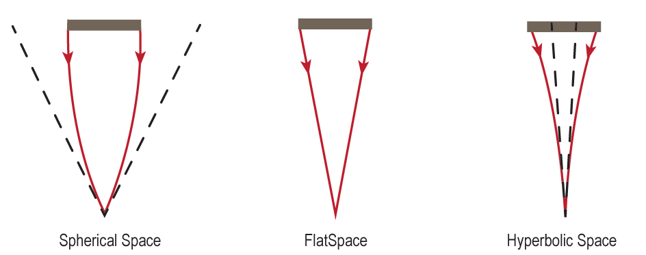
Another curved geometry is a hyperbolic geometry, in which space is saddle shaped. In such a space parallel lines diverge and the angles of a triangle add up to less than 180 degrees. This type of space is said to have negative curvature.

The shortest distance between two points is not a straight line in curved spaces. The more general name for the shortest distance between two points is a geodesic. In a flat space, a geodesic is a familiar straight line. An example of a geodesic on a curved surface is a great circle on the surface of Earth—like lines of constant longitude. A great circle is the route an airplane flies between two cities because it is the shortest distance between them. That is why flights from North America to Europe generally pass over the Arctic. Have a look at an Earth globe and you will see that the shortest distance between the United States and Europe does indeed pass over the Arctic. To map out a great circle route, put a string on a globe at two points (say, your hometown and a distant place you might like to go on vacation—Rome, maybe, or Tahiti). On a globe the string will stretch directly from the beginning to the end of your journey, but the route will look curved when projected onto a flat map of Earth such as the one in the in-flight magazine on your trip. Figure 15.14 illustrates spherical, flat, and hyperbolic spaces.

Figure 15.14: Geometry in spherical, flat, and hyperbolic spaces. In a spherical space, lines that start off as parallel eventually intersect. In flat space, parallel lines stay parallel. In a hyperbolic space, lines that start off as parallel eventually diverge. Credit: NASA/SSU/Aurore Simonnet

If spacetime is curved, light from an object will follow the curvature of spacetime; it will travel along a geodesic. Thus an object will appear to be a different angular size depending on how space is curved. This is analogous to looking at yourself in a fun house mirror or a car mirror that says “objects may be closer than they appear,” both of which have curved surfaces that distort the images they produce. Unlike the case of a mirror, in which the light travels straight paths and only the curvature of the reflecting surface gives us the distortions we see, when space itself is curved it is the curved path of the light as it travels that causes the distortions. If space is positively curved, an object will appear bigger to us than the same object seen in a flat space. If space is negatively curved, an object will appear smaller than if space is flat. Figure 15.15 illustrates the path of light in spaces of various curvatures.

Figure 15.15: The path of light from an object to an observer in (a) space which is positively curved, (b) space which is not curved and (c) space which is negatively curved. An object of a given size appears bigger in a positively curved space and smaller in a negatively curved space than in a space that is not curved. Credit: NASA/SSU/Aurore Simonnet

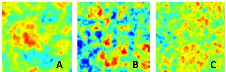
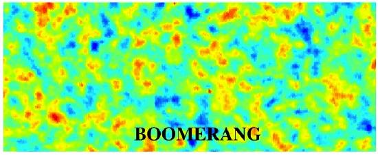
One of the ways we can measure the curvature of the Universe is through anisotropy in CMB; the hot and cold spots in the CMB would appear bigger in a spherically curved Universe than in a Universe that is not curved. In 2000, the BOOMERANG Collaboration used this technique to determine the geometry of the Universe. In the next activity, you will compare their data to three theoretical possibilities in order to determine the overall curvature of the Universe.

Determining the Geometry of Space

In this activity you will compare CMB data from BOOMERANG with theoretical models in order to determine whether the geometry of the Universe is spherical (positive curvature), flat (zero curvature), or hyperbolic (negative curvature).

A. Comparing Maps

Figure A.15.2 shows three theoretical possibilities for how the CMB anisotropy pattern might appear in a map of the sky depending on the curvature of the Universe.

Figure A.15.2: Simulated maps of the CMB differ based on the geometry of the Universe. Credit: BOOMERANG Collaboration.

1.

2.

3.

4.

Figure A.15.3 shows the BOOMERANG data. We can compare it with the models.

Figure A.15.2 to determine the overall curvature of the Universe. Credit: BOOMERANG Collaboration.

5.

B. Dependence of the Power Spectrum on Curvature

Figure A.15.4 shows three theoretical possibilities (plotted as lines) for how the CMB anisotropy power spectrum might appear depending on the curvature of the Universe.

Figure A.15.4: The CMB power spectrum changes depending on the geometry of the Universe; in particular, the angular scale of the first peak shifts. Larger I values correspond to smaller angular scales. Three theoretical models are shown: spherical (pink), flat (blue), and hyperbolic (green). Credit: NASA/SSU/Aurore Simonnet. Models run with CAMB software through NASA’s LAMBDA interface.

1.

2.

3.

4.

C. Comparing Power Spectra

Figure A.15.5 shows the CMB power spectrum as measured by BOOMERANG.

Figure A.15.5: BOOMERANG measurement of the CMB power spectrum . Credit: NASA/SSU/Aurore Simonnet based on BOOMERANG data from deBernardis et al. (2000), Nature, 404, 955.

1.

2.

 

In the last activity, you should have determined that overall, the Universe is not curved, it is flat. The BOOMERANG result of zero curvature has since been confirmed by a number of other observations, including some made with much more sensitive instruments, to better than 0.5% precision! Again, the technical term for “not curved” is “flat.” This does not mean two-dimensional, like a pancake; the Universe has at least three spatial dimensions. “Flat” also does not mean thicker in any particular dimension, it just means not curved. Stars, galaxies, and other objects still curve space locally, but these CMB observations indicate that globally, space is not curved.