15.4: Understanding the Variations in the CMB

Learning Objectives

• You will understand why the universe became transparent when the CMB formed
• You will understand acoustic oscillations

What Do You Think: What Causes the Variations in the CMB

Out of the relatively smooth early Universe formed the lumpy Universe that we see today, with its galaxies, clusters and stars. How did this happen?

The Big Bang theory doesn’t tell us how structures formed in the Universe, but it does provide a context in which they can form. We discussed how, once the Universe had cooled enough so matter and light stopped interacting strongly, the photons were free to travel freely through space. At the same time, the atoms were freed as well. For the first time, baryonic matter was able to begin clumping into what would become the structures we see today, falling into and enhancing the dense regions already occupied by the dark matter.

The CMB is the link between the smooth early Universe and the lumpy older one. As we saw in Section 15.3, while the CMB is overall remarkably uniform, there are slight variations in its temperature, called anisotropy. These temperature variations correspond to variations in the density of matter in the Universe at the time that the CMB formed. In the CMB anisotropy maps we have shown, blue spots correspond to colder, denser regions, and red spots to hotter, less dense regions. The temperatures, and therefore the densities from place to place are only different from each other by a tiny fraction: 10–100 parts per million.

The seeds for the variations in the CMB were produced early in the history of the Universe as a by-product of the fact that the vacuum of space is not really empty. Energy is constantly appearing and disappearing in the form of particles that pop rapidly into and out of existence, a concept confirmed by laboratory experiment. These quantum fluctuations very early in the history of the Universe could have been the tiny seeds of structure that became the variations in the CMB and eventually the large-scale collections of galaxies that we see today. The tiny energy fluctuations could have been expanded to very large proportions during an early epoch of rapid expansion.

Before the formation of the CMB at an age of 380,000 years, before electrons combined with nuclei to form neutral atoms, the Universe was a soup of baryons (protons and neutrons), leptons (electrons and neutrinos), and photons. Oscillations much like sound waves in this primordial fluid were created by the pressure of photons resisting gravitational compression of the plasma. Variations in the density of the primordial soup from one place to another affected the temperature of the plasma, and therefore the light; regions of compression and rarefaction at the time the CMB formed correspond to cold and hot spots. As described above, the reason the denser regions appear colder in a CMB map is because denser regions have a stronger gravitational field. The CMB photons lose some energy escaping from that gravitational pull, and therefore have a longer wavelength, which corresponds to a lower temperature.

The exact anisotropy pattern produced depends on cosmological parameters, much like the tone quality of a musical instrument depends on the materials from which it is composed. For example, the amount of baryonic matter in the Universe, including both the luminous and dark baryonic matter, cannot by itself produce sufficient gravitational attraction to allow the small variations in density to grow to the density of galaxy structures. For this reason there must be non-baryonic matter, specifically cold dark matter, present. Without the cold dark matter we cannot explain the level of anisotropy in the CMB.

If the Universe was made only of baryonic matter we would see a different anisotropy pattern in the CMB. The reason for this is that while the baryonic matter and light were interacting strongly, the pressure of the light prevented the baryons from forming dense structures. This was not true for the dark matter because it does not interact with light. Dark matter was able to begin to collapse even while the light and regular matter were strongly coupled—assuming its temperature was cold enough for it to do so. Thus the seeds of our current structures were planted even while atoms were prevented from creating any structures. By examining the observed CMB anisotropy pattern, we can place limits on the amount of baryonic matter and cold dark matter in the Universe.

One of the ways we can examine the CMB is with a map, but another technique allows us to measure temperature differences at each angular scale. This is done by computing a power spectrum of the data (or map). The power spectrum is like a filter on the map. It describes how common variations in temperature with different angular sizes are on the sky. Scientists could express this in terms of the angle itself, but mathematically it is more efficient to give each angular scale a multipole number, l. Small values of l correspond to large angular scales (some greater than a degree) and larger values of l correspond to small angular scales (some much less than a degree). Animated Figure 15.11 shows how a map can be filtered at different angular scales to create a power spectrum.

Figure 15.11: A map of the CMB can be decomposed into different angular scales, to create a power spectrum. Credit: Wayne Hu

The measured power spectrum in the sky is then compared to model power spectra that are computed for different values of cosmological parameters; some have more or less matter, others have different global geometry for the Universe, or they have varying values for the initial density fluctuations, etc. By varying all the different parameters it is possible to create a model with an impressively good fit to the data. Figure 15.12 shows the power spectrum and model fit for the Planck data, taken in 2013. The power spectrum peaks at an l of about 200 or an angular scale of about 1 degree. That angular scale is the most prominent scale in the Planck map, i.e. most of the spots are about a degree in size.

Figure 15.12: Power spectrum of the Planck anisotropy data. The data points are shown with error bars in red and the best fit model is shown in green. The Planck data are exquisitely precise and cover a wide range of angular scales. Credit: ESA and the Planck Collaboration

How Cosmological Parameters Affect the CMB

Going back to our musical analogy, the angular scales (l number) in the power spectrum are like musical tones. The power spectrum for the CMB is different depending on the contents of the Universe, similar to how the note “C” sounds different on a trombone and saxophone, because they are made of different materials.

In this activity you will explore how changing the amount of regular matter and dark matter affects the CMB power spectrum. When you play the activities, adjust the amounts by using the slider.

A. Regular Matter

1.

Play Activity

2.

B. Cold Dark Matter

1.

Play Activity

2.

3.

In the previous activity, you should have noticed several effects on the CMB power spectrum when changing the amount of regular (baryonic) matter and (exotic) cold dark matter (CDM). These changes can be explained by differences in how these types of matter interact and how structures grow. Baryons and CDM are similar in that they both have mass and therefore gravitational attraction. But only baryons interact electromagnetically. Therefore baryons, but not CDM, are part of the acoustically-oscillating fluid, along with photons and electrons.

Structures can begin to grow via gravitational attraction when they are smaller than the cosmic horizon scale. The cosmic horizon is the radius of the observable Universe, or how far light can travel based on the age of the Universe at that time. Essentially this is a size scale on which different parts of the Universe can exchange information with one another; within the cosmic horizon, all parts of the structure are able to influence each other via gravity and energy exchange. The acoustic mode corresponding to the first peak in the CMB power spectrum is the scale of the cosmic horizon size at the time the CMB formed. This marks a dividing line between what are considered “large” and “small” scales.

An important point in the history of the Universe, known as matter-radiation equality, is depicted in Figure 15.13. At this time, the density of radiation (photons) was equal to the density of matter. Before this time, radiation dominated the energy density of the Universe. Depending on the model, matter-radiation equality occurs when the Universe is about 50,000 years old. In a model with more matter, this time occurs sooner than if the amount of matter is lower.

Figure 15.13 Matter-radiation equality equality occurs when the Universe is about 50,000 years old, when the densities of matter and radiation (photons) are exactly equal. Matter-radiation equality occurs before the time when neutral atoms form and the CMB begins free streaming at 380,000 years. Credit: NASA/SSU/Aurore Simonnet

So, for example, in a model with more dark matter, matter dominates earlier, meaning photons become less important at a relatively early time. The result is a lower amplitude seen in the peaks of the CMB power spectrum. You should have observed this effect in the last activity; more CDM meant a lower power spectrum. We can explain the effects of changing the baryon fraction on the power spectrum in terms of the oscillating baryon-photon fluid. First, if we add more baryons, we notice an overall increase in the amplitude of oscillations. We also notice that odd peaks are enhanced relative to even peaks. Odd peaks in the power spectrum are associated with regions of greater density (compression). Baryons are gravitationally attracted to regions of greater density. So, if there is a greater number of baryons, odd peaks will be relatively bigger and even peaks will be relatively smaller compared to the case of fewer baryons.

Finally, you may have noticed some subtle shifts of the power spectrum at large l values (small scales) where the power is dropping off. This part of the power spectrum is known as the damping tail. Damping of the oscillations occurs on scales smaller than the distance photons travel during the short time the CMB formed. In the activity, you may have noticed that increasing the baryon fraction shifts the damping tail to smaller scales (bigger l). Increasing the amount of cold dark matter shifts the damping tail to larger scales (smaller l) by increasing the age of Universe at the time neutral atoms form.

For further reading on the physics of how the CMB works, see Wayne Hu’s CMB Tutorials.

Going Further 15.2: CMBPolarization

Light is a wave. It is made up of oscillating electric and magnetic fields. These fields have both a strength and a direction. In electromagnetic waves, the electric and magnetic fields always point in a direction perpendicular to the direction the wave travels. They also are perpendicular to each other. See Figure B.15.3 for an illustration of the geometry.

Figure B.15.3: Schematic of an electromagnetic wave. An electromagnetic wave traveling in some direction, taken here to be the z-axis, has an electric field (E, in blue) that points along the x-axis and a magnetic field (B, in brown) that points along the y-axis. The fields oscillate up and down but always remain perpendicular to each other and to the direction the wave travels. If an electron is sitting near the origin, it will feel a force as the wave passes, oscillating up and down. Credit: NASA/SSU/Aurore Simonnet

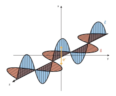
In Figure B.15.3 there is an electron depicted sitting near the origin. When a light wave passes by as shown, the electron will feel a force from the electric field in the wave. It will alternately be pushed up and then down along the x-axis, oscillating with the passing wave. An electron bouncing up and down will radiate electromagnetic waves - accelerated charged particles always emit electromagnetic waves. The emitted waves will have the same frequency at which the electron oscillates, and in this case that is the same frequency as the incident wave. The energy radiated by the electron must come from somewhere, and the only source of energy the electron has is the incident light wave. So what the electron is doing is absorbing some of the energy of the incident wave and re-radiating it in different directions. We call this scattering.

In the case that we have described here, scattering preserves the frequency of the incident wave, merely directing some of the wave’s energy into new directions. Scattering does not always preserve the frequency of the incident light- it can increase or decrease the frequency depending on the details of the scattering material (whether it is hot, cold, in motion, etc.). We discussed this type of scattering in Going Further 15.1: The Sunyaev-Zel’dovich (SZ) Effect.

Now we will examine the direction of scattered light. The intensity of the electromagnetic waves radiated by the electron (in other words, scattered by the electron), will depend on the amplitude of the motion of the electron as seen by an observer in that direction. For instance, if you are an observer sitting somewhere in the y-z plane, you will see the electron move up and down to its full extent, and the intensity of the emitted radiation will be maximal. If you are somewhere above or below the y-z plane you will see a smaller amplitude for its motion since some of the motion is directly toward or away from you, and you cannot see that. In the extreme case that you sit on the x-axis directly above or below the electron, you will not see it move at all. For such an observer the intensity of the emitted radiation is zero. In other words, there is no radiation emitted directly along the x-axis for the situation depicted.

Light is said to be polarized if the electric field only oscillates in one direction. We will now describe how scattering can polarize light. Imagine that you are an observer watching the scattering of light from the electron, and you are positioned such that your line of sight to the electron makes a 90 degree angle with the direction the wave travels, which puts you somewhere on the x-y plane. If you are aligned along the x-axis you will not see any of the scattered light from the electron because its motion is directly toward and away from you. If you are on the y-axis you will see maximum intensity for the scattered light. In other places in the x-y plane you see intermediate intensities. The geometry is depicted in Figure B.15.4.

Figure B.15.4: An electromagnetic wave, incident from the lower right, is shown in this image. Part of the wave is scattered by an electron through a 90 degree angle toward an observer. From the point of view of someone looking toward the incident wave, all orientations of the electric field are visible, as shown in the inset, at right. However, to an observer of the scattered wave, only those directions of the electric field that are perpendicular to the sightline are visible. As a result, the observer of the scattered wave sees light polarized in a direction perpendicular to the direction of travel of the incident wave. Credit: NASA/SSU/Aurore Simonnet

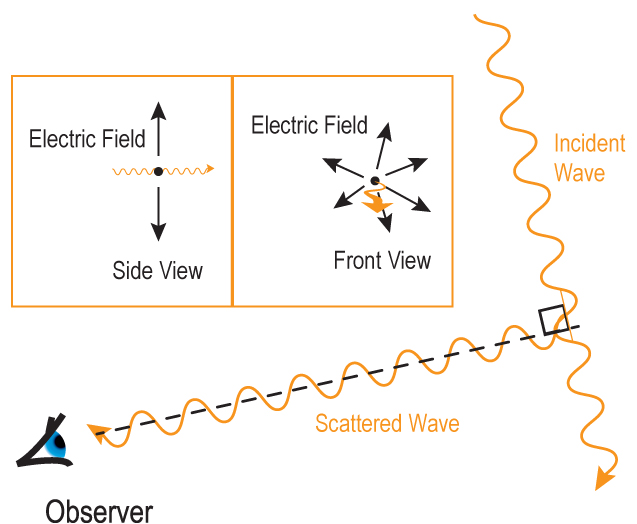
What is interesting about the geometry described is that the light you see will always have its electric field along the x-axis. Since the incident light is propagating in the z-direction, there is no component of the electric field for the incident ray in that direction, so the electron does not move in that direction. It can move along the y-direction, but if you are on the y-axis you cannot see that motion. The scattered light you see therefore will have only one direction for its electric field, no matter what the direction of the electric field of the incident light. Another way to think about this is that it does not matter how the x and y axes are aligned with respect to the incident light wave: as long as you can see some light it will be polarized.

You can see this effect in the daytime sky on Earth, just look at the sky in a region about 90 degrees away from the Sun using polarized sunglasses. Tilt your head slightly. You will see the intensity of the sky change as the polarized filters in the glasses block more or less of the light, depending on the orientation of the filters and the electric field in the scattered sunlight.

When light his a preferential orientation for its electric (and magnetic) field, we say it is polarized. The process of scattering tends to polarize light. Of course, there is a lot of scattered light in Earth’s atmosphere, so when you look at a point in the sky there will generally be light coming from different directions, with only a fraction coming directly from the Sun. That is why the sky does not become totally dark when you look at it through polarized sunglasses. However, the incident light itself is not polarized. Different waves have different orientation of their electric fields, and it is only the process of scattering that polarizes the light.

This same scattering process occurred early in the Universe as the CMB was being produced. In general, at any given point there was light coming from all directions. This is a different situation from the case of sunlight in the atmosphere, where there is a preferential direction toward the source (the Sun). The polarization of light from one direction with be cancelled by the polarization of light coming from directions 90 degrees away, and so no net polarization occurs under this circumstances. However, there is a possible way to break the symmetry and get a net polarization of the scattered radiation.

To understand where this net polarization comes from, imagine that the fluid containing the scattering electrons is moving relative to the frame of the CMB. In the direction of the motion of the fluid the photons will be blueshifted, and in the direction opposite the motion the radiation will be redshifted by the same amount. In intermediate directions the redshift and blueshift will be less, with no shift occurring in directions perpendicular to the direction of motion of the fluid. This introduces an asymmetry in the radiation field. Alone, it does not produce a net polarization of scattered radiation. The incoming radiation from the forward direction, which has higher than average intensity due to its blueshift, causes scattered radiation with higher than average intensity. On the other hand, the incoming radiation from the backward direction, which has equally diminished intensity because of its redshift, creates scattered radiation with lower than average intensity. The two scattered components combine to give a net intensity that is identical to the average, and so no net polarization is seen. The same is true for directions oblique to the direction of motion: radiation from opposite sides of the sky combine to give no net polarization.

Now consider what happens if the electron is in a place where the gas on one side is falling toward it and the gas on the opposite side is also falling toward it (Figure B.15.5). In perpendicular directions the gas can be stationary, moving away or moving inward at a slower speed . Given any of those scenarios, the scattering electron will see hot spots in two opposite directions and (relatively) cool spots in directions 90 degrees from those. Now the light incoming from the hot spots does not average out to give the typical temperature since the radiation from both directions has a higher intensity than the average. Similarly, light coming in from the cool places gives a lower intensity. Thus an observer looking at this region will see a polarization signal with either a slightly higher than average temperature or a slightly lower than average temperature, depending on how the gas was moving when the microwave light was emitted and the relative direction to the observer.

Figure B.15.5 CMB Polar Producer. This gives an idealized view of what the sky looks like to an electron that could produce polarized light in the CMB. The electron is imagined to be in the center of this shape. Along two directions opposite in the sky, the blue bubbles here, the temperature would appear hotter than average. In perpendicular directions, illustrated with a red torus, the sky would be cooler than average. This is one example of a temperature configuration, from the perspective of the electrons scattering the light, which would cause a net polarization in the scattered waves. Credit: NASA/SSU/Aurore Simonnet

This is a powerful technique. It allows astronomers to determine if the gas that created the CMB was collapsing in some places and expanding in others, and it gives them detailed information about how that collapse was occurring in different parts of the sky and on different angular scales. Since our theories of structure formation depend on gas collapsing into high density regions to form the structures we now see as galaxy clusters and filaments, careful observations of the polarization of the CMB give us important checks on these theories.

The polarization signal is quite weak. Power spectra of CMB polarization data are at levels about 100 times lower than CMB temperature anisotropy, where fluctuations are already at a level of 1 part per 10,000. Operating from the South Pole, DASI was the first group to detect polarization in the CMB in 2002. CMB polarization has since been detected by several other groups.

Finally, the polarization of the CMB is also sensitive to a small percentage of the Universe being ionized once stars started forming. This tells us that the first stars must have turned on around a redshift of around 10, when the Universe was about 400 million years old.

Going Further 15.3: the Steady State Theory Cannot Explain the CMB

In searching for your own understanding of the Universe, you can weigh the observational evidence for the Big Bang plus structure formation model presented in this module.

Here we will compare the explanatory power of the Big Bang theory with that of the Steady State theory. The Big Bang theory incorporates a beginning to the Universe as well as its evolution. An alternative, the Steady State theory, was proposed in 1948 by Hermann Bondi, Thomas Gold, and Fred Hoyle. The Steady State theory also incorporates the expanding Universe. Clusters of galaxies move farther apart over time, and the spaces between them enlarge. To keep the Universe looking the same, new matter, which condenses into new galaxies, must continually be created within the spaces. We cannot rule out such creation with laboratory tests. To fill the space left by the expansion of the Universe requires that three or four new atoms appear per year per cubic kilometer . A cubic kilometer of air at sea level contains 1037 atoms, rendering the few new ones completely undetectable.

How can we discriminate between the two theories? The Big Bang theory predicts the cosmic microwave background as the cooled remnant of the hot, dense phase of the early Universe. The Universe therefore appears to be changing with time. This conclusion is also supported by the observed evolution of galaxies and quasars as we look to distant and therefore younger reaches of the Universe. Though to be fair, Steady State models generally did not accept the common interpretation of the cosmological redshift, and so the evolution of the quasar population could be circumvented, though in a way that failed to convince most astronomers.

Steady State cosmologies had particular difficulty explaining the CMB, as there is no reasonable way to explain the perfect blackbody spectrum of the radiation observed in all directions. The CMB was thus seen as the death knell for Steady State cosmological models. Since that time evidence has accumulated for the evolution of the galaxy population and large scale structures in the Universe, both of which are incompatible with an unchanging Universe. Essentially no one takes Steady State models seriously anymore.