17.3: The Friedmann Equation and the Fate of the Universe

Some say the world will end in fire,

Some say in ice.

From what I’ve tasted of desire

I hold with those who favor fire.

But if it had to perish twice,

I think I know enough of hate

To say that for destruction ice

Is also great

And would suffice.

WHAT DO YOU THINK: FATE OF THE UNIVERSE

Some students are contemplating the end of the Universe.

• Bo: I think the Universe will keep expanding and cooling, galaxies will keep pulling farther apart from each other, and eventually everything will be dark.
• Candice: I don't think it makes sense to expand forever. I think the expansion will only go for so long, then it will begin to contract because of gravity . I think it’s going to reach a maximum, then collapse back onto itself.
• Dante: It strikes me that the Universe ought to be timeless and that the Universe is just expanding and collapsing perpetually.
• Emily: No, I think Bo is right, except I think it’s supposed to eventually expand so much that everything gets ripped apart.
• Feng: I don’t think there’s any way to know or predict the fate of the Universe.

Do you agree with any or all of these students and, if so, whom?

Bo

Candice

Dante

Emily

Feng

None

Explain.

 

THE FRIEDMANN EQUATION

The basis to understanding how the expansion of the Universe can be speeding up lies in the Einstein equations. General relativity can tell us physically what factors relate to the expansion. One version of the Einstein equations is the Friedmann equation, which describes how the expansion rate changes over time, and why, in a homogeneous and isotropic Universe.

\[\color{red}H^2\color{black}-\color{green}\dfrac{8\pi G\rho}{3}\color{black}= \color{blue}\dfrac{kc^2}{S^2} \nonumber \]

\[\color{red}(expansion)\color{black}-\color{green}(density)\color{black}= \color{blue}(curvature) \nonumber \]

In this equation, H is the Hubble parameter (expansion rate), ρ is the average density of matter and energy in the Universe, S is the scale factor, and k is a number that describes the overall curvature of the Universe. That means the expansion is related to the contents of the Universe as well as the curvature of space.

The density term includes all of the types of matter and energy in the Universe.

\[\rho =\rho_{baryon} + \rho_{cdm} + \rho_{radiation} + \rho_{DE} \nonumber \]

Here \(\rho_{baryon}\) is the density of regular matter (baryons), \(\rho_{cdm}\) is the density of cold dark matter, \(\rho_{radiation}\) is the density of radiation, and \(\rho_{DE}\) is the dark energy density.

The Friedmann equation embodies the essence of the Einstein equation: matter and energy affect how spacetime bends. In general relativity, it is not only matter that produces curvature, but any sort of energy. This means that the gravitational attraction has a contribution not just from regular matter, but also from dark matter and radiation (massless particles like photons). The kinetic energy of particles is generally included in the Einstein equations as a pressure term, because pressure can be thought of as an energy density, or a kinetic energy per unit volume. There is also negative pressure from dark energy.

There is a special value of the density that causes the Universe to have zero curvature. It is called \(\rho_{crit}\), the critical density:

\[ρ_{crit}=\dfrac{3H^2}{8\pi G} \nonumber \]

If the current density is equal to the critical density, then the left side of the Friedmann equation equals 0, implying that k = 0. We say that such a Universe has no curvature, or that it is flat.

Math Exploration 17.1: Calculating the Critical Density

Worked Example:

1. What is the value of the critical density?

We can calculate \(ρ_c\) using a Hubble constant of H₀ = 70 km/s/Mpc. The value of the gravitational constant is G = 6.67 x 10^-11 m³/kg s².

• Given: H₀ = 70 km/s/Mpc, G = 6.67 x 10^-11 m³/kg s²
• Find: \(ρ_c\)
• Concepts:
  • ρ_c = 3H²/(8πG)
  • 1 Mpc = 3.086 × 10¹⁹ km
• Solve:

\[\rho_c=\frac{3(70~\rm{km/s/Mpc})^2}{8\pi\left(6.67\times10^{-11}~\rm{m^3/kg~s^2}\right)} \nonumber \]

Now we need to do some unit conversions:

\[\rho_c=\frac{3{\left(70~\frac{km}{s\cdot Mpc}\times\frac{1~Mpc}{3.086\times10^{19}km}\right)}^2}{8\pi\left(6.67\times10^{-11}\frac{m^3}{kg\cdot s^2}\right)} \nonumber \]

Solving and simplifying units, we get:

\[\rho_c=3.07 \times 10^{-27}kg/m^{3} \nonumber \]

In the Friedmann equation, only the ratio of density to the critical density is important. This ratio is so important that it is given its own name: Ω (Greek letter “omega”):

\[\Omega\equiv \dfrac{ρ}{ρ_{crit}} \nonumber \]

In general relativity, all of the sources of matter and energy are included and contribute to the total energy density. Thus we have:

\[\Omega=\Omega_{baryon} + \Omega_{cdm} + \Omega_{radiation} + \Omega_{DE} \nonumber \]

Here \(\Omega_{baryon}\) is the baryon content, \(\Omega_{cdm}\) is the amount of cold dark matter, \(\Omega_{radiation}\) is the radiation content, and \(\Omega_{DE}\) is the contribution from dark energy.

If \(\Omega = 1\), that means the density is equal to the critical density, so we have a flat Universe (k = 0).

We will generally discuss the density and geometry of the Universe in terms of \(\Omega\) from now on rather than in terms of k or \(ρ_{crit}\). One of the major efforts in cosmology over the past several decades has been to determine the value of \(\Omega\).

From the Friedmann equation, we can see that the interplay of the expansion of the Universe, density, and curvature lead to several possibilities for the fate of the Universe, depending on which term in the equation dominates:

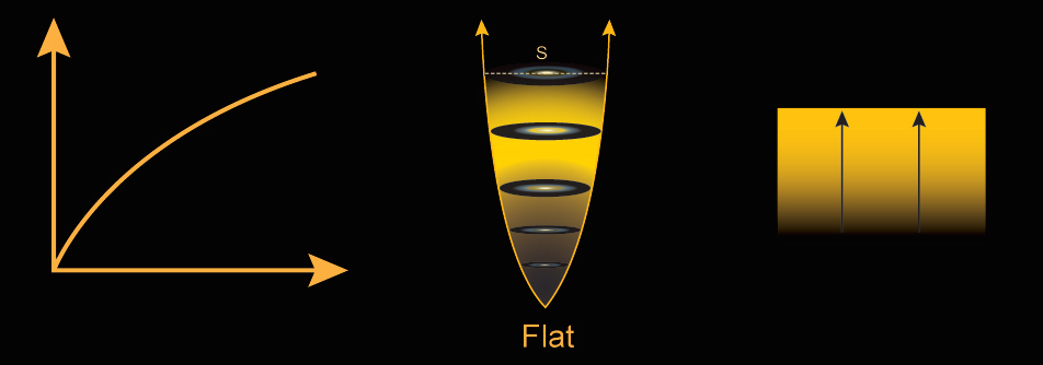
1. Critical Universe: We have already discussed the case of a critical Universe, where the expansion and density terms are equal, \(\Omega = 1\), and space overall is not curved. If there is no dark energy, the Universe will continue to expand, but increasingly slowly.
2. Matter terms dominate: If the Universe contains enough mass to counteract its expansion and there is no dark energy, it will eventually collapse. This is known as a closed Universe. In this case, \(\Omega > 1\).
3. Expansion term dominates: If the Universe does not contain enough mass to counteract its expansion and there is no dark energy, it will expand forever. This is known as an open Universe. In this case, \(\Omega < 1\).
4. Dark energy dominates: None of the three possibilities above lead to the accelerating expansion rate supported by supernova data. Dark energy can cause the expansion to speed up; therefore, we must examine possibilities that include dark energy.

We will consider each of these in detail next. We will explore how the expansion rate changes over time, what the matter-energy density (\(\Omega\)) is like in each case, the resulting curvature of space, and what conditions in the Universe will be like in the future. First, we will consider the three scenarios with no dark energy, then we will explore scenarios that include dark energy.

THE UNIVERSE WITHOUT DARK ENERGY

The interplay between the terms of the Friedmann equation can be compared to the interplay between gravity and the energy of motion for a ball rising into the air using Newtonian physics.

Case 1: A Critical Universe

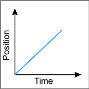
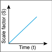
First, consider a scenario where a ball is launched at escape velocity from Earth’s surface. The kinetic energy from the ball’s motion exactly equals its gravitational potential energy. In other words, the sum of the terms for motion and gravity is zero. In this case, the ball will continue to fly away from Earth, but at an ever slower rate. This is analogous to a critical Universe. In a critical Universe the expansion (motion) and density (gravity) terms of the Friedmann equation sum to zero. The motion diagram for a ball at escape speed (position vs. time) and a diagram for the scale factor vs. time in a critical Universe are compared in Figure 17.4.

Figure 17.4: Left: a ball is launched from Earth at escape velocity (which is found by setting kinetic and potential energies equal to one another). The ball continues to move away from Earth, but at increasingly slower speeds, as shown by the flattening slope of the graph. Right: The scale factor of the Universe in the case of critical density. The expansion and gravity terms in the Friedmann equation are equal. The Universe continues to expand, but at an increasingly slower rate, as shown by the flattening slope. Credit: NASA/SSU/Aurore Simonnet.

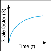
In general relativity, the curvature of space as a whole is related to the expansion and gravity terms. In the case of a critical Universe, the curvature is zero. The expansion and geometry for a critical Universe are depicted in Figure 17.5.

Figure 17.5: The expansion and geometry for a critical Universe. Left: A graph of the scale factor vs. time. Center: An illustration showing that the Universe continues to expand but ever more slowly. Right: The geometry of the Universe is flat, in other words, there is no curvature in any of the three spatial dimensions. Credit: NASA/SSU/Aurore Simonnet

In a critical Universe, space will continue to expand. As it expands, it will cool endlessly, approaching a temperature of 0 K (—273°C). It is at 2.7 K already, and as the temperature drops, the motions of particles and molecules will slow down. Stars will eventually burn out. Galaxies will run out of gas to make any new stars. No energetic photons will be produced to keep things warm. Collisions between particles will be too lethargic to excite electrons, and those collisions will become less and less frequent as the density drops. Black holes will eventually evaporate, and some particles thought currently to be stable might decay to simpler forms. Eventually, physical processes will simply cease, after unimaginably long timescales in excess of 10¹⁰⁰ years. The fate of the Universe in this case is known as a big chill (Animated Figure 17.6).

@api/deki/files/54210/LinearExpansion.mp4?origin=mt-web < video src=”@api/deki/files/54210/LinearExpansion.mp4” type=”video/webm” controls > < /video >

 

 

Animated Figure 17.6: In a big chill scenario, galaxies continue to move away from each other forever, as the Universe expands and cools. Credit: NASA/SSU/Kevin John

Case 2: A Closed Universe

Now consider a case where a ball is launched from Earth’s surface, but with less kinetic energy. In that case, the ball will rise to a certain height and then fall back down to the ground because the gravitational potential energy overwhelms the energy of motion. This is analogous to what happens if the density of matter is greater than that required to produce a flat Universe. In that case, gravity will overwhelm the expansion of the Universe and it will eventually stop expanding and re-collapse. The density is greater than critical (\(\Omega > 1\)). The left side of the Friedmann equation is negative, implying that the curvature is positive. That is the case for a closed Universe. The motion diagram (position vs. time) for a ball launched at less than escape speed and a diagram for the scale factor vs. time in a closed Universe are compared in Figure 17.7. The expansion and geometry for a critical Universe are depicted in Figure 17.8.

Figure 17.7 Left: A ball is launched from Earth at slower than escape velocity. At first it moves away from Earth, but then it reaches a maximum height and falls back down due to gravity. Right: The scale factor of the Universe in the case of a closed Universe. The gravity term in the Friedmann equation outweighs the expansion term. At first the Universe expands, but then it contracts due to gravity. Credit: NASA/SSU/Aurore Simonnet.

Figure 17.8 The expansion and geometry for a closed Universe. Left: A graph of the scale factor vs. time. Center: An illustration showing that the Universe expands then contracts. Right: The curvature of the Universe as a whole is positive, or in other words, the geometry of the Universe is spherical. Note that this means the global geometry is analogous to that of a sphere. It does not mean that the Universe is a sphere. Credit: NASA/SSU/Aurore Simonnet.

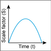
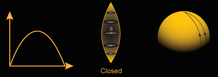
In a closed Universe, space will expand for a while but eventually stop and begin to collapse in upon itself, heating as it does so. Galaxies will move toward each other and the temperature of the Universe will increase. The particles in galaxies will eventually merge together into a state of high temperature and density similar to that found in the beginning of the Universe. The fate of the Universe in this case is known as a big crunch. It is depicted in Animated Figure 17.9.

Animated Figure 17.9 In a big crunch scenario, the gravitational attraction of matter causes galaxies to eventually start moving toward each other and the Universe becomes more dense. Credit: NASA/SSU/Kevin John.

Case 3: An Open Universe

At the opposite extreme, when the density of the Universe is less than critical (\(\Omega < 1\)), the gravity will never be able to halt the expansion. This is analogous to a ball launched from Earth with a speed greater than escape speed; the kinetic energy of the ball can overcome the gravitational pull from Earth. The motion diagram (position vs. time) for a ball launched with kinetic energy greater than its gravitational potential energy and a diagram for the scale factor vs. time in a closed Universe are compared in Figure 17.10.

Figure 17.10 Left: A ball is launched from Earth at a speed greater than escape velocity. It flies away from Earth because its kinetic energy is greater than its potential energy. Right: The scale factor of the Universe in the case of an open Universe. The expansion term in the Friedmann equation outweighs the gravity term and the Universe expands forever at a constant rate. Credit: NASA/SSU/Aurore Simonnet.

In the case of an open Universe, the left side of the Friedmann equation is positive, so the curvature must be negative. That happens when the curvature of the Universe is saddle-shaped. The expansion and geometry for an open Universe are depicted in Figure 17.11. In an open Universe, space will continue to expand. In a fate similar to that of the critical case, galaxies will move farther apart from each other, the temperature of the Universe will cool, and stars in galaxies will eventually burn out. Again, we would have a big chill scenario.

Figure 17.11 The expansion and geometry for an open Universe. Left: A graph of the scale factor vs. time. Center: An illustration showing that the Universe expands forever. Right: The curvature of the Universe as a whole is negative, or in other words, the geometry of the Universe is saddle-shaped (hyperbolic). Credit: NASA/SSU/Aurore Simonnet.

From these three cases—open, closed, and critical—we can see that changing the amount of matter in the Universe changes the way it expands. A lot of matter means that the cosmic expansion cannot overcome the gravitational attraction of the matter. The expansion could eventually slow until it stops, and then the Universe will re-collapse. On the other hand, if there is not enough matter in the Universe, then the expansion continues forever. These two cases are separated by a condition in which there is just enough matter for expansion to balance gravity—the critical case.

If no dark energy is present, once we determine the value of the curvature, we know it forever. It represents the geometry of the Universe as a whole. This is true whether the matter in the Universe is baryons or cold dark matter (or a combination of both). The Friedmann equation alone determines whether the Universe keeps expanding forever or eventually re-collapses; whether the scale factor S grows or shrinks is determined here only by the density of the Universe, which also determines its overall geometry.

EXPANSION OF THE UNIVERSE DEPENDS ON MATTER DENSITY

In the simplest cosmological models, the fate of the Universe depends on its rate of expansion, expressed by the Hubble parameter, and the amount of matter it contains. Qualitatively, the Hubble constant gives us an idea of the kinetic energy associated with the expansion of space. The matter content gives us an idea of the gravitational potential energy. In a Newtonian context, the two taken together give us the total energy. In general relativity, they produce the total curvature of the Universe.

In this activity, you will be allowed to adjust \(\Omega\) and take note of how the expansion varies as this parameter changes.

Play Activity

1. In which scenario does the Universe eventually collapse?

Ω < 1

Ω = 1

1"> Ω > 1

2. In which scenario does the Universe expand at a constant rate forever?

Ω < 1

Ω = 1

1"> Ω > 1

3. In the Ω = 1 case, the graph of scale factor vs. time is a straight line.

True

False

EXPANSION AND GEOMETRY OF THE UNIVERSE

For the questions below, refer to Figure A.17.8, which shows three possible scenarios for the expansion of the Universe and the geometry that goes with them.

Figure A.17.8 Three different scenarios for the expansion of a matter-only Universe. On the left are graphs of the scale factor vs. time, in the center are illustrations depicting the scale factor of the Universe as time advances, and on the right are models for the curvature of space. Each scenario corresponds to a different curvature. Top row: positive curvature, the Universe expands for a while, then stops expanding and eventually collapses. Center row: zero curvature, the Universe expands forever but increasingly slowly. Bottom row: negative curvature, the Universe expands at a constant expansion rate forever. Credit: NASA/SSU/Aurore Simonnet.

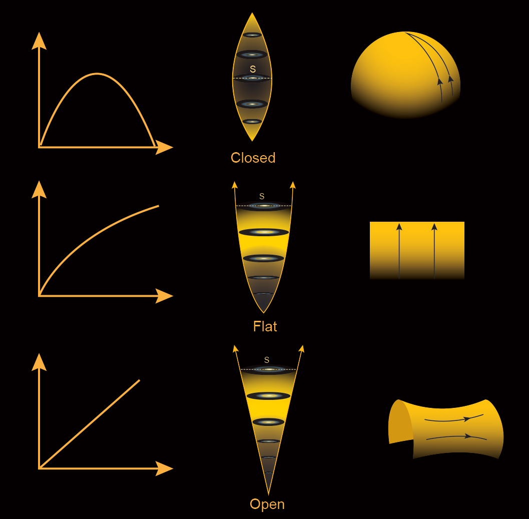
1. Which scenario features negative curvature?

Top row

Center row

Bottom row

2. Which scenario shows a flat Universe?

Top row

Center row

Bottom row

3. Which scenario shows a Universe with positive curvature?

Top row

Center row

Bottom row

4. Which scenario features a Universe that expands forever, but increasingly slowly?

Positive curvature

Zero curvature

Negative curvature

5. In which scenario does the Universe expand at a constant rate forever?

Positive curvature

Zero curvature

Negative curvature

6. In which scenario does the Universe eventually collapse?

Positive curvature

Zero curvature

Negative curvature

In the previous activity, you saw that the Universe will either expand forever or eventually stop expanding, depending on how much mass it contains. In two of the cases, the expansion slows over time. The slowing is the result of the gravitational attraction that all the mass in the Universe has for all the other mass. The slowdown means that the age of the Universe is not simply the reciprocal of the Hubble constant, 1/H_0, as would be the case for a constant expansion rate. In the next activity, you will examine how the matter density and expansion rate affect the age of the Universe.

EXPANSION SCENARIO AND AGE OF THE UNIVERSE

In this activity, we will explore how changing the amount of matter and the expansion rate affects the age of the Universe for a closed Universe scenario.

The age of the Universe will be the amount of time that passes between the beginning of the Universe and the point at which the scale factor again becomes zero (blue line intersects the x-axis).

Play Activity

1. What happens to the age of the Universe if the Hubble constant (expansion rate) is greater?

The age is greater.

The age is less.

The age does not change.

2. What happens to the age of the Universe if the density (Ω) is greater?

The age is greater.

The age is less.

The age does not change

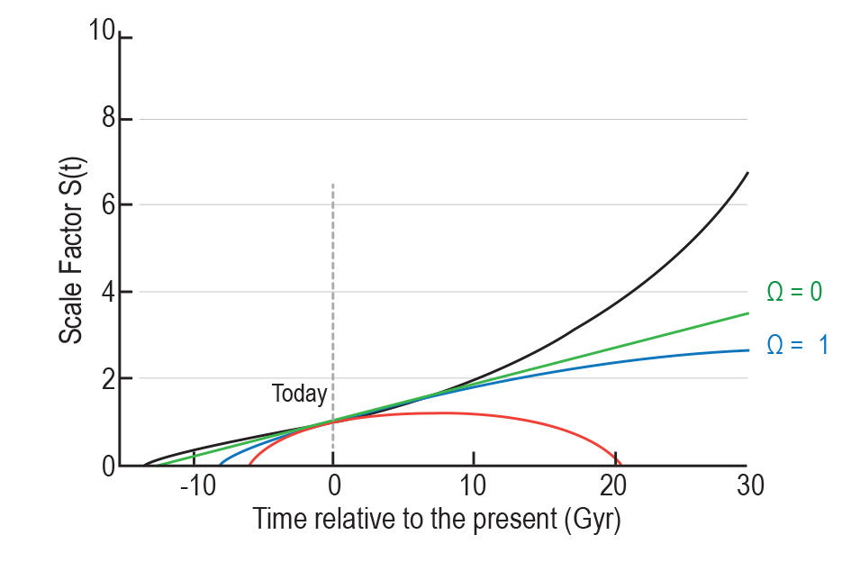
In the previous activity, you saw how changing the value of the expansion rate and density affected the age for a closed Universe. Figure 17.12 shows how the scale factor changes with time in the closed, open, and critical cases. It also shows what would happen in a case where the expansion is accelerating. We can see that the age of the Universe (time from the beginning until “now”) is smallest for a closed Universe and increases as \(\Omega\) gets smaller. Physically, this is because the age of the Universe is inversely proportional to the expansion rate; if the Universe expands more quickly, it takes less time to reach the state it is in today. If \(\Omega > 1\), the expansion rate was greater in the past than it is today; thus the age will be younger compared to a Universe with constant expansion. The reverse is true if the expansion rate is speeding up.

Figure 17.12 Several different possibilities for the age of the Universe. The red curve represents a closed Universe (\(\Omega > 1\)), which is the youngest possibility (about 7 billion years). As the density decreases, the age of the Universe today increases. For example, for a flat Universe with no dark energy as seen in the blue curve (\(\Omega = 1\)), the age of the Universe would be about 9 billion years; for a Universe devoid of matter (green curve) the age would be even greater. The greatest age for the Universe occurs in a Universe with an accelerating expansion due to dark energy (black curve). In this case, the age of the Universe matches observations (13.8 billion years old), further evidence that the Universe contains dark energy. Credit: NASA/SSU/Aurore Simonnet.

UNIVERSE WITH DARK ENERGY

In the previous section, we looked at how changing the amount of matter in the Universe relates to its expansion, age, and overall geometry. We saw a variety of outcomes, but none of them predicted an accelerating expansion. For that, we need dark energy. Including dark energy can cause dramatically different outcomes for the age, geometry, and eventual fate of the Universe, as compared to cases without dark energy. The exact outcome depends on the nature of the dark energy. There are three interesting dark energy scenarios: the dark energy could be a cosmological constant, it could grow stronger, or it could grow weaker.

In the case of dark energy being a cosmological constant (\(\Lambda\)), its density is constant—it is a property of space itself. Over time its contribution to the total energy density (\(\Omega\)) increases because there is more and more space (containing a constant amount of \(\Lambda\) per unit volume). On the other hand, the total amount of matter and radiation is fixed. As the expansion progresses they become more and more dilute. In the next activity, you will see how in this scenario the total density to change over time, and how its constituent parts contribute different amounts at different eras in the evolution of the Universe.

BEHAVIOR OF DENSITY OVER TIME

In this activity you will explore how the proportions of radiation, matter, and dark energy (called \(\Omega_R\), \(\Omega_M\), and \(\Omega_D\), respectively) change over the history of the Universe. They are represented as fractions of the overall matter—energy budget in a cosmic pie chart. Here, we assume that the dark energy takes the form of a cosmological constant.

Use the slider bar to adjust the redshift (\(z\)) and answer the following questions.

Play Activity

1. When we look at higher redshift (z), we are (choose all that apply):

Looking farther back in time

Looking at the Universe earlier times in its history

Looking at later times in its history

Redshift is not related to time

2. What happens to the proportion of radiation as redshift gets bigger?

It is bigger

It is smaller

It remains the same

3. At what redshift were the proportions of radiation and matter approximately equal to each other?

z =

 

4. Was this before, after, or at the same time as the formation of the CMB (z ~ 1100)?

Before

After

Same time

5. Around what redshift do we start to see dark energy making up part of the matter-energy budget?

z =

 

6. Dark energy is what percentage of the matter-energy budget today?

 

%

As time advances from the past until now, the redshift gets smaller and the scale factor (S) gets larger. In the last activity, you should have seen that the energy contribution from matter and radiation as a percentage of the cosmic matter-energy budget both diminish, while the percentage of dark energy increases. The contribution from matter drops as 1/S³ because the particles are being spread over a greater volume as the Universe expands. The radiation contribution shrinks faster than matter because in addition to the number of photons per unit volume dropping (like the number of baryons and dark matter particles), the photon energy is also decreased due to the cosmological expansion; as the light shifts to longer wavelengths, the energy per photon drops. Thus, the total energy contribution from radiation decreases like 1/S⁴. Dark energy (if interpreted as a cosmological constant) remains a constant number as the scale factor increases and thus becomes a greater percentage of the matter-energy budget.

We can write this mathematically if we express the total density in terms of the scale factor.

\[\rho(S)=\rho_{crit}\left [\Omega_{DE}+\dfrac{\Omega_M}{S^3}+\dfrac{\Omega_R}{S^4}\right ] \nonumber \]

The scale factor here is S, \(\rho_{crit}\) is the current critical density, \(\Omega_{DE}\) is the amount of dark energy, \(\Omega_M\) is the amount of matter, and \(\Omega_R\) is the amount of radiation. We can also demonstrate how this equation works in Figure 17.14, where we show how each of the densities (radiation, matter, and dark energy) drop as time advances.

Figure 17.13 Energy density vs. time. The black line shows the decrease in the energy density of matter, and the red line shows the decrease in the energy density of radiation. The blue line shows the constant energy density of dark energy when it is assumed to be in the form of a cosmological constant (although other possibilities have not been completely ruled out). Earlier times in the history of the Universe are to the left and later times are to the right. Today is zero on the x-axis. Credit: NASA/SSU/Aurore Simonnet based on Frieman, Turner, and Huterer 2008. Annual Reviews in Astronomy and Astrophysics, 46, 385.

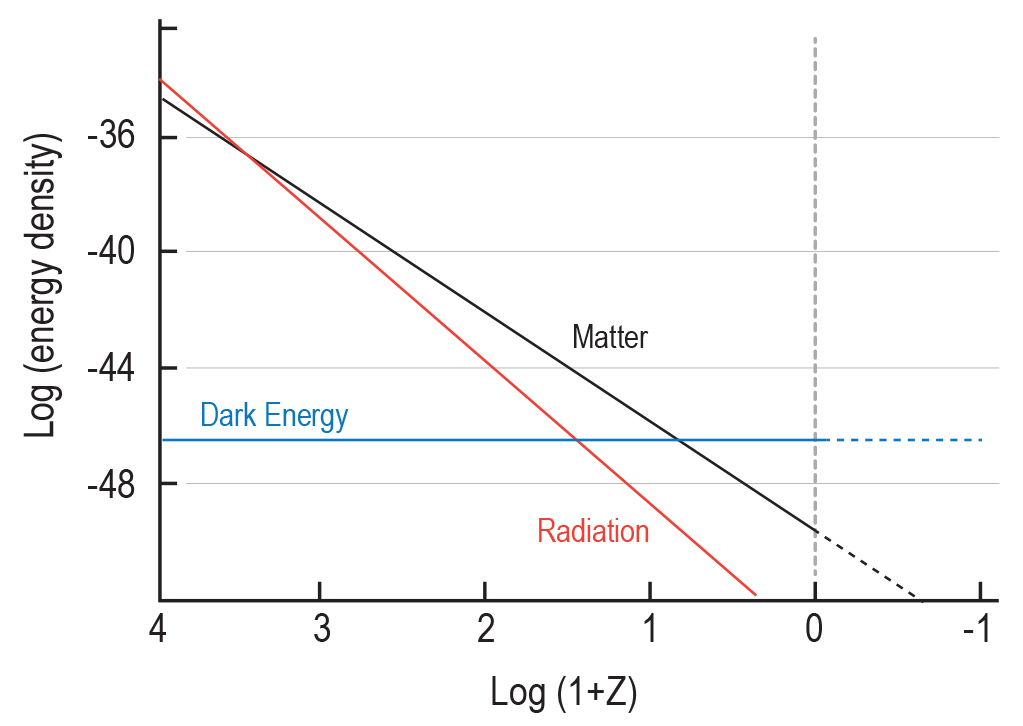
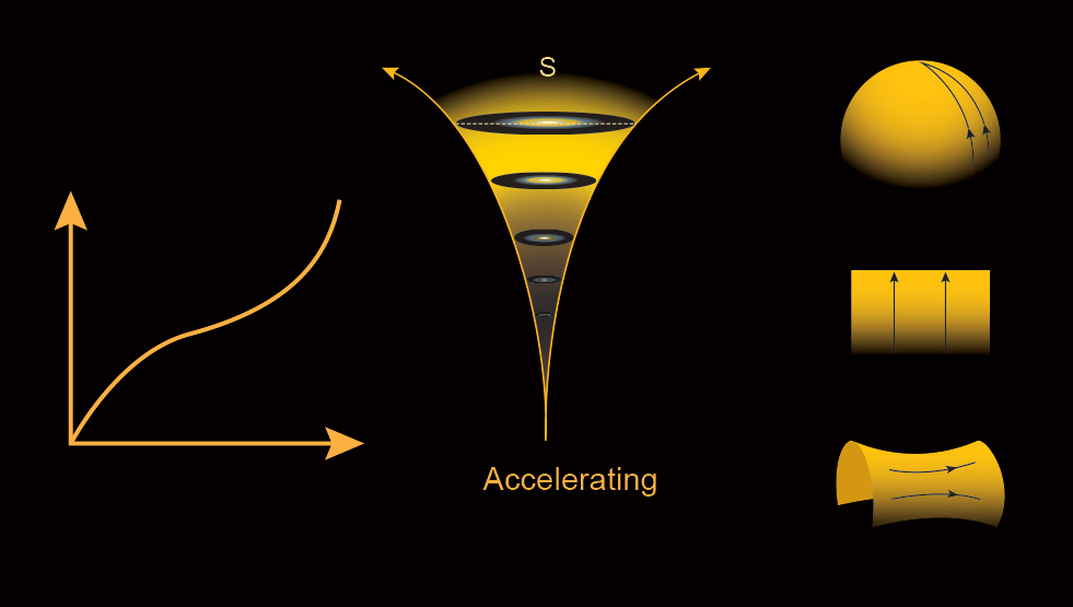
As we can see from Figure 17.13, dark energy (in the form of a cosmological constant) remains unaffected by the expansion. As dark energy becomes more dominant, it makes the expansion speed up, and objects in the Universe begin to accelerate away from each other. In a Universe with a cosmological constant, we will have a big chill scenario, plus an additional interesting effect. Galaxies will move away from each other increasingly quickly such that eventually an observer in any galaxy will see all galaxies outside her own small region disappear over her cosmic horizon. The only objects visible will be the ones in her own galaxy and possibly a few bound neighbors such as those in the Local Group of the Milky Way. This is a slow-motion recapitulation of what is thought to have occurred during the inflationary period in the early Universe.

The expansion of the Universe in a scenario with a cosmological constant is depicted schematically in Figure 17.14. Unlike a matter-only Universe, one with \(\Lambda\) will eventually speed up, no matter the initial curvature.

Figure 17.14 In a Universe that contains both matter and dark energy, it is possible for the expansion rate to accelerate with time. In some models, the dark energy can increase with time, in others it remains constant, while in others it may eventually decrease. In order to predict the eventual fate of the Universe, we need to understand more about the properties of dark energy. Credit: NASA/SSU/Aurore Simonnet.

The nature of the dark energy is still not settled. Increasing evidence indicates that it is indeed a cosmological constant, a constant property of space like the vacuum energy. However, other possibilities have not been completely ruled out; dark energy could change over time, becoming either stronger or weaker.

If the strength of the dark energy grows in time, and not only as a proportion of the total energy density like the cosmological constant, the dark energy concentration per unit volume increases. The increase in density will lead to an exponential expansion of space like the one that caused inflation early on. Eventually, the dark energy will become so strong that the expansion will tear galaxies apart. It will even rip molecules, atoms, and protons apart as its strength grows without bound. This scenario is referred to as the big rip (Animated Figure 17.15).

Animated Figure 17.15 In a big rip scenario, galaxies continue to move away from each other forever, as the Universe expands and cools. Dark energy that grows in strength causes the expansion to accelerate so strongly that eventually galaxies and even atoms to be ripped apart. Credit: NASA/SSU/Kevin John.

Finally, the dark matter might have a decreasing density and becomes less important with time. In this case, the expansion of the Universe would continue forever, but at a continually slowing rate, a scenario qualitatively similar to a Universe with no dark energy at all. In fact, that is what such a Universe eventually becomes as its dark energy density approaches zero.

Table 17.1 summarizes the possible scenarios for the fate of the Universe, both with and without dark energy.

Table 17.1 Possible scenarios for the fate of the Universe in the Big Bang model

SCENARIO	DOMINANT TERM	MATTER DENSITY	CURVATURE	OUTCOME
Critical (No Dark Energy)	None	Ωm = 1	Zero (flat)	Big Chill
Closed (No Dark Energy)	Matter	Ωm > 1	Positive (like a sphere)	Big Crunch
Open (No Dark Energy)	Expansion	Ωm < 1	Negative (like a saddle)	Big Chill
Dark Energy Constant	Dark Energy	could be any and still get acceleration at some point	could be any and still get acceleration	Big Chill
Dark Energy Increases	Dark Energy	could be any and still get acceleration at some point	could be any and still get acceleration	Big Rip
Dark Energy Decreases	Dark Energy and then Matter	depends on specific model	could be any and still get expansion	Big Chill

The Big Bang model not only tells us where we have come from, it also predicts where we are going — in the cosmic sense. The model explains observations of the state of the Universe in the past and the present, and it also predicts what will happen to the Universe in the future. The Big Bang model gives us insight into questions like: Will the Universe expand forever? Will it stop expanding and then collapse? The Big Bang model and general relativity tell us each of those scenarios is possible, and they predict specifically what the Universe will be like in each of them. They also tell us how to determine which scenario will occur based on quantities we can measure today.

So, what is the fate of our Universe? Will it expand forever, endlessly cooling to the point of a “big chill,” will it eventually reverse its direction and collapse into a “big crunch,” or will dark energy grow in strength enough to cause a “big rip?” In the next section, we will see how a combination of different observations has helped astronomers answer these questions.