17.4: Cosmic Concordance and Cosmological Parameters

WHAT DO YOU THINK: WHAT IS THE MOST IMPORTANT EVIDENCE FOR THE BIG BANG?

Some students are studying for their cosmology class.

• Gabe: Here, in my notes, it says the main evidence for the Big Bang theory is Hubble’s discovery of the expansion of the Universe.
• Hans: What about the cosmic microwave background? I think that’s just as important. Maybe even more important.
• Ilse: And how much there is of each element. I think that’s important for the Big Bang.
• Jerome: I think it’s the large-scale structure, like how galaxies and the cosmic web formed.
• Kitty: I still think astronomers just make this stuff up.

Do you agree with any or all of these students and if so whom?

Gabe

Hans

Ilse

Jerome

Kitty

None

Explain.

THE CONCORDANCE MODEL: PUTTING THE MEASUREMENTS TOGETHER

Our current understanding of the formation and subsequent evolution of the Universe rests not on a single observation, but on a host of independent observations. It has extended beyond the original Big Bang model, which envisioned only that early on the Universe was in a hot and dense state. Our current theory of cosmology includes ideas like inflation, formation of large-scale structures, the cosmic microwave background (CMB) and its fluctuations, the creation of light elements, and other aspects of the Universe. The current overall theory of the formation and evolution of the cosmos is able to explain not only the early hot, dense state, but also how structures were able to form from that early state. Our best current model of the Universe is referred to as the concordance model. In this section we show how the various cosmological parameters in the theory fit together with multiple lines of observational evidence. We will also highlight areas where work still has to be done to complete our understanding.

In the early versions of the Big Bang theory, the quantities of concern were the expansion rate of the Universe (H₀), the existence of relic thermal radiation (the CMB), and the overall geometry of the Universe as described by the overall density parameter (\(\Omega\)). As observations and our understanding have become more sophisticated, our theories have as well. Now our ideas encompass the baryon fraction (\(\Omega_{baryon}\)), the baryon-to-photon ratio (\(\eta\)), the density of cold dark matter (\(\Omega_M\)), the dark energy fraction (\(\Omega_{DE}\)), and other quantities. Some model parameters are familiar and have already been discussed. Others are fairly technical for a non-expert; indeed, cosmologists add new parameters as the observations become more precise and are able to distinguish small differences between models.

What we would like to illustrate is how several independent observations can work together to place strong limits on the models, eliminating some possibilities and increasing our confidence that the concordance model is a good description of the Universe. We should repeat here that all of our conclusions have as their underpinnings the Friedmann—Robertson—Walker idea of a homogeneous and isotropic Universe described by general relativity. In this framework, small local deviations from the global homogeneity eventually lead to the structures we see in the present Universe.

Supernova data provided the first evidence that the Universe contained dark energy. Shortly afterward, the first precise measurements that determined the geometry of the Universe (and therefore \(\Omega\)) were the measurements of the tiny temperature variations in the CMB. Repeated measurements by a variety of ground and space-based instruments have confirmed that the Universe is flat, that is, that the sum of all the matter-energy density in the Universe is the critical value, or in the language of cosmological researchers, \(\Omega=1\). (See Going Further 17.2: The Flat Universe).

GOING FURTHER 17.2: A FLAT UNIVERSE

Our best measurements of large-scale structure indicate that the total amount of matter - both baryonic and dark - accounts for about 30% of the critical amount. Therefore, the rest must be something else. Dynamically, we are missing about 70% of the energy content of the Universe, though these measurements do not give any hint about what that 70% might be. That is evidence for some energy density that we cannot see dynamically on the scales of galaxies and galaxy clusters. These observations point to, but do not necessarily demonstrate, the existence of dark energy.

The hot and cold spots we observe in the CMB, and the cosmic web of large-scale structures that we see throughout the Universe today, both formed from high- and low-density regions in the early Universe. The delicate looking cosmic web of galaxies, galaxy clusters, and filaments connecting them, form differently under the influence of dark energy than they do if no dark energy is present. Indeed, even different forms of dark energy can affect the eventual structures that exist later in the Universe.

While we have only one Universe to observe and study, we can model it using sophisticated computations. We can calculate many different instances of cosmic evolution to see how structure formation differs under different conditions. We then compare the output of the models to the structures that we observe. In these models, astronomers can vary, for example, the amounts of dark energy, dark matter, baryonic matter, radiation, the size of initial cosmic fluctuations and several other parameters.

One of the observable predictions of the models is the size and spacing of large-scale structures. Another is the spectrum of CMB variations. When cosmologists compare their models to the actual Universe, some of the most robust conclusions they find is that the structures we see are consistent with models that contain dark energy, and that they are inconsistent with models that do not contain dark energy. Furthermore, without dark matter there is not enough time for the structures we see to form. To learn more about why, see Going Further 17.3: Why CMB and Large-Scale Structure Models Require Dark Matter and Dark Energy.

Different measurements have different abilities to determine cosmological parameters. For instance, measurements of the CMB by itself are not able to determine the Hubble constant independently of the geometry (\(\Omega\)) of the Universe. The two can be constrained together, but their individual uncertainties are correlated, as shown in Figure 17.16. As you can see, there are many combinations of values for the Hubble constant and \(\Omega\) that are allowed by the data. This sort of behavior is called degeneracy.

Figure 17.16 This figure shows the degeneracy in CMB data between measurements of the Hubble constant (in units of 100 km/s/Mpc: h = H₀/100) and the density of matter (Ω_m). The yellow ellipse denotes the region of 68% confidence and the green region is 95% confidence for WMAP data combined with all other CMB experiments; the inner solid contour is 68% confidence and the outer solid contour is 95% confidence for WMAP alone. (A 95% confidence contour is one in which the true value should lie outside the contour only 5% of the time. In other words, we are 95% confident that the true value lies inside the region bounded by the contour.) Credit: NASA/SSU/Aurore Simonnet based on Planck 2013 Results XVI: Cosmological Parameters, accepted to Astronomy and Astrophysics.

In order to break the degeneracy between two variables, we need additional information. Such information can be provided by a different technique that measures the same two parameters in a different way. Often this will break the degeneracy because the uncertainties for the other dataset are complementary to those of the first. Figure 17.17 illustrates the case where different measurements of the same parameters from different techniques can be combined to narrow the overall measurement uncertainties.

Figure 17.17 A single measurement of a cosmological parameter is often not able to constrain that parameter well. There may be dependencies on another parameter that create ambiguities between the two. By measuring the parameter via several methods these ambiguities, called degeneracies, can be removed in many cases. Credit: NASA/SSU/Aurore Simonnet based on Planck 2013 Results XVI: Cosmological Parameters, accepted to Astronomy and Astrophysics.

CONSTRAINING COSMOLOGICAL PARAMETERS

In this activity, you will practice simultaneously determining the fraction of matter in the Universe (Ω_m) and the Hubble constant from two different relations.

A. CMB temperature data

The pattern of temperature fluctuations in the CMB as measured by the Planck satellite can be used to measure the matter content and the Hubble constant. Unfortunately, there is a degeneracy in the two quantities such that:

\[Ω_mh^{3}=0.0959±0.0006 \nonumber \]

Here, we are writing the Hubble constant such that H₀ = 100h km/s/Mpc (in other words, h = 0.7 for H₀ = 70 km/s/Mpc, h = 0.6 for H₀ = 60 km/s/Mpc, etc.). As Ω_m goes up, the value of h must go down to keep the product constant.

For now, we will ignore the uncertainty (±0.0006) and use this relation to plot Ω_m vs. h.

1. Fill in the table below using the relationship between Ω_m and h from CMB temperature fluctuations:

Worked example:

• Given: h = 0.5
• Find: Ω_m
• Concept: Ω_m h³ = 0.0959
• We can rewrite this as: Ω_m = 0.0959/h³
• Solve: Ω_m = 0.0959/(0.5)³ = 0.767

h	\(\Omega_m\) = 0.0959h^-3
0.5	0.7672
0.6
0.7
0.8
0.9
1.0	0.0959

2. Now enter the points in the table into the plotting tool.

• Under “Dataset Controls,” click the “+” to create a new dataset
• Set the labels for the x- and y-axes to h and omega_m, respectively
• Enter the points under “Points Control”

B. Complementary data

We can get additional information about the values of Ω_m and h by using other aspects of the data. This gives a different, and complementary, constraint:

\[\Omega_m h^{−3}=1.03±0.13 \nonumber \]

To see what this means, you will plot these data on top of the data from the relationship in Part A. Again, we will ignore the uncertainty (±0.13).

1. Fill in the table below using the second relationship between Ω_m and h:

Worked example:

• Given: h = 0.5
• Find: Ω_m
• Concept: Ω_m/h³ = 1.03
• We can rewrite this as: Ω_m = 1.03 h³
• Solve: Ω_m = 1.03(0.5)³ = 0.129

h	\(\Omega_m\) = 1.03h^3
0.5	.12875
0.6
0.7
0.8
0.9
1.0	1.03

3. Now enter the points in the table into the plotting tool.

• Under “Dataset Controls,” click the “+” to create a second dataset.
• Choose a new color for this dataset
• Set the labels for the x- and y-axes to h and omega_m, respectively
• Enter the points under “Points Control”

C. Combining the data

The two curves that you have plotted are somewhat perpendicular; they cross at a point with particular values of Ω_m and h. The point where the two curves intersect is the one consistent with both datasets.

1. From your graph, what is the value of the Hubble constant?

h =

2. From your graph, what is the value of the matter fraction?

Ω_m =

In this activity, the point where the two curves intersect is the only one consistent with both datasets. In a perfect world, this would be the only consistent point, and finding its positions in the \(\Omega_m-h\) plane would determine the two parameters exactly. In the real world, we take the measurement uncertainties into account and get an ellipse that contains acceptable values, i.e., values that are consistent with both datasets.

All of our measurements contain uncertainties; it is the nature of measurement. We ignored them in the last activity, but it is possible to take them into account. To do this, we would plot a region in the \(\Omega_m-h\) plane for each relation. Instead of a line for each, we would have a region, called an error ellipse (as seen in Figures 17.16 and 17.17). The overlap of the error ellipses for the two datasets would give us a region of consistency. In this case, it would not be a point, but would have a finite size. The uncertainty associated with the measurement of each parameter is reduced by using both datasets, even if it does not disappear completely.

Astronomers combine measurements from different datasets, such as the CMB, large-scale structure, supernova distances, ages of the oldest stars, the cosmic abundance of the lightest elements, and other measurements. Each of these independent measurements has its associated uncertainties, but in general they are independent of each other. They can be thought of as complementing one another. By combining many complementary measurements together, cosmologists can narrow the overall uncertainties in all of the cosmological parameters. Table 17.2 gives the current best measurements for some of these parameters.

Table 17.2 Cosmological parameters from a simultaneous analysis of CMB temperature data from the Planck satellite, CMB temperature and polarization data from other experiments, and large-scale structure data. (Adapted from Planck 2013 Results XVI: Cosmological Parameters, accepted to Astronomy and Astrophysics.)

PARAMETER	SYMBOL	VALUE
Hubble Constant	H0	67.80 +/- 0.77 km/s/Mpc
Cold Dark Matter density	Ωcdm	0.1187 +/- 0.0017/h^2
Baryon density	Ωbaryon	0.02214 +/-0.00024/h^2
Cosmological constant density	ΩDE	0.692+/-0.010

GOING FURTHER 17.3: WHY CMB AND LARGE-SCALE STRUCTURE MODELS REQUIRE DARK MATTER

FURTHER EVIDENCE FOR DARK ENERGY

The concordance model is often called ΛCDM, because multiple measurements point to a Universe that contains not just regular matter, but also cold dark matter and dark energy; the dark energy is represented as the cosmological constant Λ, though dark energy might not actually be constant.

As we have discussed earlier, the first evidence for the presence of dark energy came from observations of Type I supernovae. But because dark energy creates an effect opposite to that of gravity, its presence should also be detectable in the way that structures form in the Universe. As a result, there should be small, but discernable, differences between a Universe composed of only matter, which condenses via gravity to form clumps, and a Universe with matter and dark energy. This is because dark energy opposes gravitational attraction and impedes the formation of clumps. If the dark energy is extremely strong, then no clumps will form at all. If it is quite weak, we will not be able to observe its effects. Clearly, in our Universe, the dark energy has not prevented the formation of structure, and astronomers have been able to search for its imprint on the structures they observe.

In Figure 17.18, we show the error ellipses from three independent data sets. The diagonal orange region is derived from CMB measurements. The blue region comes from supernova measurements. The nearly vertical green region shows results from large-scale structure measurements, specifically baryon acoustic oscillations (see Going Further 17.4: Baryon Acoustic Oscillations). Together, the three data sets place strong limits on the cosmological model. In this case the values of \(\Omega_m\) (total matter content) and \(\Omega_{DE}\) (dark energy content) are strongly constrained. The diagonal line running from upper left to lower right indicates a flat Universe, in which \(\Omega = \Omega_m + \Omega_{DE}=1\).

Figure 17.18 This plot shows constraints on the matter fraction (Ω_m) and dark energy fraction (Ω_DE) as derived from measurements of large-scale-structure baryon acoustic oscillations (BAO, green), the cosmic microwave background (CMB, orange), and supernovae (SNe, blue). None of the measurements alone does a very good job of constraining either parameter, but together they place very strong limits on both, as indicated by the gray region at their intersection. Credit: Supernova Cosmology Project, Suzuki et al. 2012, Astrophysical Journal. 746, 85.

There is something truly remarkable about this process. Different sorts of measurements — each using different kinds of instruments to look at completely different kinds of objects, all involving different kinds of physical processes — give completely consistent results. Their error ellipses converge to a small region in the parameter space. One could imagine them giving radically different answers, totally inconsistent with one another. In that case we would know that our model cosmology—the concordance model—was completely wrong. The fact that all the disparate measurements are instead convergent in a small region of parameter space lends confidence that the model is actually a fair description of the Universe and its evolution.

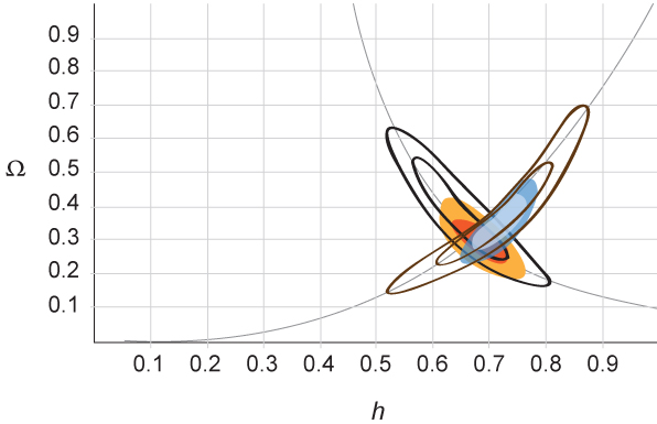
There are many complementary sets of parameters of this sort. Figure 17.19 shows an example of constraints on the dark energy from measurements of the CMB. CMB measurements are sensitive to not only the dark energy, but also the amount of normal matter (baryons, \(\Omega_{baryon}\)), the amount of cold dark matter (\(\Omega_{cdm}\)), and other parameters. These variables are shown along with the dark energy fraction, here called \(\Omega_{\Lambda}\). Error ellipses are determined from the Planck and WMAP missions. Notice how the baryon graph complements the cold dark matter graph, as their uncertainty ellipses are nearly perpendicular. Together they provide much tighter constraints on the cosmological model. Plots with other variables can also be constructed, as can plots using datasets other than those from the CMB.

Figure 17.19 The baryon fraction (Ω_bh²) and cold dark matter fraction (Ω_ch²) are plotted vs the dark energy fraction (here called Ω_Λ) from CMB data. The smaller red contours are from Planck and WMAP polarization data. The larger gray contours are from WMAP alone. The colored dots depict different values of the Hubble constant, running from 64 km/s/Mpc (blue) to 72 km/s/Mpc (red). The horizontal band running through the most likely values for the various parameters shows that they are all consistent with dark energy making up about 70% of the total energy density. The two plots complement one another because the uncertainties in one are perpendicular to the uncertainties in the other. Credit: NASA/SSU/Aurore Simonnet. —Adapted from Planck 2013 Results XVI.

GOING FURTHER 17.4: BARYON ACOUSTIC OSCILLATIONS

OBSERVATIONAL TESTS: WHAT IS THE MOST LIKELY FATE OF THE UNIVERSE?

Current observational tests of cosmology indicate that the matter in the Universe accounts for approximately 30% of the critical density. Only one-sixth of that amount is baryons. The rest is dark matter, which so far is completely undetectable aside from its gravitational influence on the baryonic material we are able to see. In addition, 70% of the matter—energy density of the Universe is dark energy. The balance of observational evidence suggests that the dark energy is a cosmological constant, though other models have not been completely ruled out. The overall curvature of the Universe is consistent with zero to high precision. Thus, the flat Universe predicted by inflation is borne out by observations. In this section, we will recap these observations with an emphasis on their cosmological ramifications.

Astronomers have long known that there is not enough matter in the Universe to create a flat geometry. They know this from their census of galaxies and galaxy clusters. From these counts they can compute a baryon density, since galaxies glow from the light of their stars. Clusters of galaxies glow from stars too, as well as from x-rays emitted by the hot intracluster gas they contain. The mass contained in this gas actually exceeds that in stars as a proportion of the total cluster mass. Of course, the bulk of the total mass in galaxies and clusters is not baryons at all, it is cold dark matter.

Outside of galaxies and clusters, a few baryons are found in the intergalactic medium. This material can be seen because it absorbs some of the light from background quasars.

When you add all of the mass - baryonic and dark matter - you find that you have \(\Omega_m = 0.3\), just under a third of what is needed for a flat geometry. This was the best that could be done until the late 1990s.

While many cosmologists were busy searching for matter in the Universe, a small group was engaged in trying to piece together the matter content by determining its expansion history. As we have already discussed, they used white dwarf supernovae to create Hubble diagrams. By using extremely bright standard candles, like Type I supernovae, these diagrams could stretch back billions of years.

To their astonishment, and almost everyone else’s, what they found was that the Universe is expanding more rapidly now than it did in the past. It therefore contains some sort of dark energy, a substance that has negative pressure. In the context of general relativity, such a substance creates a repulsive gravitational effect. The early supernova studies were not able to determine the amount of the dark energy, nor could they discern its type. But they did show that it was present in amounts significant enough to have an effect on the expansion.

About a year after the discovery of dark energy, a balloon-borne CMB experiment in Antarctica (BOOMERANG) was able to measure the first peak of the power spectrum of temperature fluctuations in the cosmic microwave background. From these data it was clear that we live in an \(\Omega = 1\) Universe. This result did not come as a surprise; inflation had made a strong prediction that the Universe must be flat, and the combination of previous CMB measurements pointed in that direction. However, directly measuring a flat geometry was an important observational test.

The \(\Omega = 1\) result, coupled with \(\Omega_m = 0.3\) from earlier studies, was an independent, though indirect, detection of the dark energy. It showed that the dark energy comprised around 70% of the critical density. Since that time, CMB measurements have also constrained the fraction that baryons (4.5%) and cold dark matter (25%) can contribute to the overall density. Subsequent CMB experiments of much higher sensitivity have also confirmed and strengthened the \(\Omega = 1\), \(\Omega_{DE} = 0.7\) finding.

In addition to these measurements, the first decade or so of this century has seen cosmologists increase their efforts to understand the details of the Big Bang paradigm and the concordance model. One of the most powerful methods they have employed has been to use galaxy redshift surveys to extract the three-dimensional distribution of matter in the Universe. Just like the CMB, the pattern of fluctuations in the data is intimately related to the constituents of the Universe: it is the same density fluctuations in the early Universe that formed the hot and cool spots in the CMB and the high- and low-density regions that are seen as galaxy clusters, filaments, and voids today.

Unlike the CMB, the galaxy distribution can be studied at different times by observing galaxies at different redshifts. When this is done, it allows cosmologists to observe effects like the dark energy as it begins to dominate the expansion. These sorts of studies have not only confirmed that the dark energy exists, but they strongly imply that it is a constant in time, a cosmological constant rather than other models in which dark energy varies in time.

Thus, our current understanding suggests that the Universe will eventually cool in a big chill, with an expansion rate that is ever increasing. Dark energy began to dominate the energy content of the Universe around six to eight billion years after the Universe began, and the overall composition is increasingly dominated by dark energy. This is depicted in Figure 17.20.

The conclusion of a dark energy-dominated cosmology is still not completely certain, but most data suggest that is where the Universe is headed. The expansion and geometry of the Universe according to our current best measurements is depicted schematically in Figure 17.21 and Animated Figure 17.22. Time will tell if this is the correct picture, or if important modifications will be necessary as new data are collected and analysed.

Figure 17.20 Current data suggests that the dark energy is a cosmological constant. Therefore, as the Universe continues to expand, the dark energy will come to dominate more and more, driving the expansion to ever-faster rates. Under these conditions, the Universe eventually reaches a big chill scenario. Credit: NASA/SSU/Aurore Simonnet.

Figure 17.21 The concordance model of the Universe. With the inclusion of dark energy, a flat Universe will undergo accelerating expansion. The graph on the left is the scale factor vs. time, which is illustrated in the center. The illustration on the right indicates that the geometry of the Universe is flat, in other words, that the curvature of space overall is zero. Credit: NASA/SSU/Aurore Simonnet.

Animated Figure 17.22 Current data indicates that expansion of the Universe will speed up due to dark energy, and that the fate will be a big chill scenario. Credit: NASA/SSU/Kevin John.