10.6: Rotational Broadening

The lines in the spectrum of a rotating star are broadened because light from the receding limb is redshifted and light from the approaching limb is blueshifted. It may be remarked that early-type stars (type F and earlier) tend to be much faster rotators than later-type stars, and consequently early-type stars show more rotational broadening. It should also be remarked that pole-on rotators do not, of course, show rotational broadening (even early-type fast rotators).

I shall stick to astronomical custom and refer to a “redshift” as a shift towards a longer wavelength, even though for an infrared line a “redshift” in this sense would be a shift away from the red! A “longward” shift doesn’t quite solve the problem either, for the following reason. While it is true that relativity makes no distinction between a moving source and a moving observer, in the case of the Doppler effect in the context of sound in air, if the observer is moving, there may be a change in the pitch of the perceived sound, but there is no change in wavelength!

We shall start by considering a star whose axis of rotation is in the plane of the sky, and which is of uniform radiance across its surface. We shall then move on to oblique rotators, and then to limb-darkened stars. A further complication that could be considered would be non-uniform rotation. Thus, the Sun does not rotate as a solid body, but the angular speed at low latitudes is faster than at higher latitudes – the so-called “equatorial acceleration”.

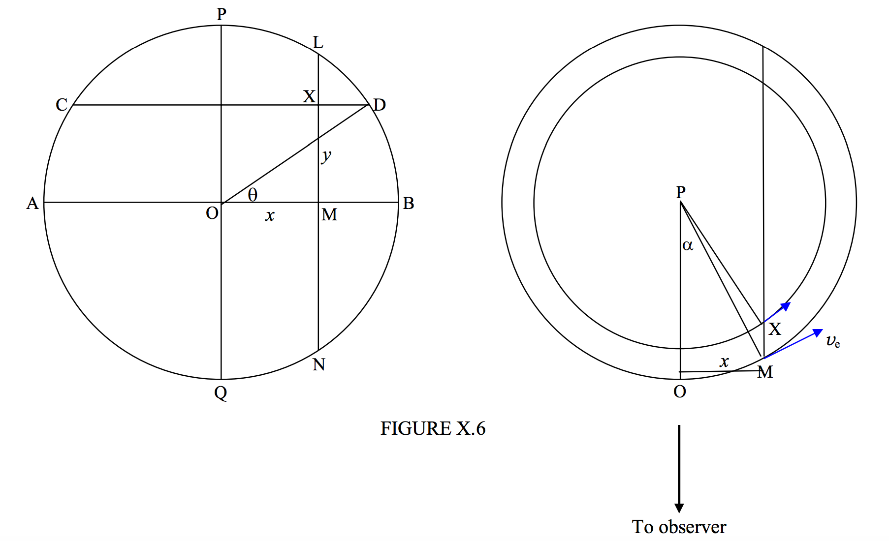
In figure X.6, on the left hand we see the disc of a star as seen on the sky by an observer. PQ is the axis of rotation, supposed to be in the plane of the sky, and AB is the equator. X is a point on the surface of the star at coordinates $(x, y)$, latitude $\theta$. The star is supposed to be rotating with an equatorial speed $v_e$. What we are going to show is that all points on the chord LMN have the same radial velocity away from or towards the observer, and consequently all light from points on this chord has the same Doppler shift.

The right hand part of the figure shows the star seen from above the pole P. The small circle is the parallel of latitude CD shown on the left hand part of the figure.

M is a point on the equator and also on the chord LMN. Its speed is $v_e$ and the radial component of its velocity is $v_e \sin \alpha$. The speed of the point M is $v_e \cos \theta$, and its radial velocity is $v_e \cos \theta \sin \text{OPX}$. But $x = \text{PM} \sin \alpha = a \sin \alpha\text{ and }x = \text{PX} \sin \text{OPX} = a \cos \theta \sin \text{OPX}$. Therefore $\cos \theta \sin \text{OPX} = \sin \alpha$. Therefore the radial velocity of X is $v_e \sin \alpha$, which is the same as that of M, and therefore all points on the chord LMN have radial velocity $v_e \sin \alpha = v_e x/a$.

Therefore all points on the chord $x =$ constant are subject to the same Doppler shift

$$\label{10.7.1}\dfrac{\Delta \lambda}{\lambda}=\dfrac{v_e x}{ac}.$$

The ordinate of an emission line profile at Doppler shift $\Delta \lambda$ compared with its ordinate at the line center is equal to the ratio of the length of the chord $x =$ constant to the diameter $2a$ of the stellar disk:

$$\label{10.7.2}\frac{I_\lambda \left ( \Delta \lambda \right )}{I_\lambda (0)}=\left ( 1-\frac{x^2}{a^2}\right )^{\frac{1}{2}}=\left ( 1-\frac{c^2\left (\Delta \lambda \right )^2 }{v_e^2\lambda^2}\right )^\frac{1}{2}.$$

In the above, we have assumed that the axis of rotation is in the plane of the sky, or that the inclination $i$ of the equator to the plane of the sky is $90^\circ$. If the inclination is not $90^\circ$, the only effect is that all radial velocities are reduced by a factor of $\sin i$, so that Equation $\ref{10.7.2}$ becomes

$$\label{10.7.3}\frac{I_\lambda \left ( \Delta \lambda \right )}{I_\lambda (0)}=\left ( 1-\frac{c^2\left ( \Delta \lambda \right )^2}{v_e^2 \sin^2 i \lambda^2}\right )^\frac{1}{2},$$

and this is the line profile. It is an ellipse, and if we write $\frac{I_\lambda \left ( \Delta \lambda \right )}{I_\lambda (0)}=X \text{ and }\frac{\Delta \lambda}{\lambda}=Y$ Equation $\ref{10.7.3}$ can be written

$$\label{10.7.4}\frac{x^2}{\left ( \frac{v_e \sin i}{c}\right )^2}+\frac{y^2}{1^2}=1.$$

The basal width of the line (which has no asymptotic wings) is $\frac{2v_e \sin i}{c}$ and the FWHM is $\frac{\sqrt{3}v_e\sin i}{c}$. The profile of an absorption line of central depth $d$ is

$$\label{10.7.5}\frac{I_\lambda \left ( \Delta \lambda \right )}{I_\lambda (0)}=1-d\left (1-\frac{c^2 \left (\Delta \lambda \right )^2}{v_e^2\sin^2 i\lambda^2}\right )^\frac{1}{2},$$

It is left as an exercise to show that

$$\text{Equivalent width}=\frac{\pi}{\sqrt{12}}\times \text{central depth}\times \text{FWHm}=0.9069 dw .\label{10.7.6}$$

From the width of a rotationally broadened line we can determine $v_e \sin i$, but we cannot determine $v_e\text{ and }i$ separately without additional information. Likewise, we cannot determine the angular speed of rotation unless we know the radius independently.

It might be noted that, for a rotating planet, visible only by reflected light, the Doppler effect is doubled by reflection, so the basal width of a rotationally broadened line is

$$\dfrac{4v_e \sin i}{c}. \nonumber$$

Now let us examine the effect of limb darkening. I am going to use the words intensity and radiance in their strictly correct senses as described in Chapter 1, and the symbols $I\text{ and }L$ respectively. That is, radiance = intensity per unit projected area. For spectral intensity and spectral radiance – i.e. intensity and radiance per unit wavelength interval, I shall use a subscript $\lambda$.

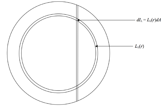
$\text{FIGURE X.7}$

We suppose that the spectral radiance at a distance $r$ from the center of the disc is $L_\lambda (r)$. The intensity from an elemental area $dA$ on the disc is $dI_\lambda = L_\lambda (r)dA$. The area between the vertical strip and the annulus in figure X.7 is a little parallelogram of length $dy$ and width $dx$, so that $dA = dxdy$. Here $y^2 = r^2 - x^2$, so that

$$dy=\frac{rdr}{y}=\dfrac{rdr}{\sqrt{r^2-x^2}}. \nonumber$$

Therefore $dA=\frac{rdrdx}{\sqrt{r^2-x^2}}$. The total intensity from the strip of width $dx$, which is $dI_\lambda (\Delta \lambda)$, where $\frac{\Delta \lambda}{\lambda}=\frac{xv_e \sin i}{ac}$, is

$$\label{10.7.7}dI_\lambda (\Delta \lambda) = 2\int_x^a \dfrac{L_\lambda (r)rdr}{\sqrt{r^2-x^2}}dx.$$

The (emission) line profile is

$$\label{10.7.8}\frac{I_\lambda (\Delta \lambda)}{I_\lambda (0)}=\dfrac{\int_x^a \frac{L_\lambda (r)rdr}{\sqrt{r^2-x^2}}dx}{\int_0^a L_\lambda (r)dr},$$

which is the line profile. As an exercise, see if you can find an expression for the line profile if the limb=darkening is given by $L_\theta =L(0)[1-u(1-\cos \theta)]$, and show that if the limb-darkening coefficient $u = 1$, the profile is parabolic.

Equation $\ref{10.7.8}$ enables you to calculate the line profile, given the limb darkening. The more practical, but more difficult, problem, is to invert the Equation and, from the observed line profile, find the limb darkening. Examples of this integral, and its inversion by solution of an integral equation, are given by Tatum and Jaworski, J. Quant. Spectr. Rad. Transfer, 38, 319, (1987).

Further pursuit of this problem would be to calculate the line profile of a uniform star that is rotating faster at the equator than at the poles, and then for a star that is both limbdarkened and equatorially accelerated – and then see if it is possible to invert the problem uniquely and determine both the limb darkening and the equatorial acceleration from the line profile. That would be quite a challenge.