1.2: Numerical Integration

There are many occasions when one may wish to integrate an expression numerically rather than analytically. Sometimes one cannot find an analytical expression for an integral, or, if one can, it is so complicated that it is just as quick to integrate numerically as it is to tabulate the analytical expression. Or one may have a table of numbers to integrate rather than an analytical Equation. Many computers and programmable calculators have internal routines for integration, which one can call upon (at risk) without having any idea how they work. It is assumed that the reader of this chapter, however, wants to be able to carry out a numerical integration without calling upon an existing routine that has been written by somebody else.

There are many different methods of numerical integration, but the one known as Simpson's Rule is easy to program, rapid to perform and usually very accurate. (Thomas Simpson, 1710 - 1761, was an English mathematician, author of A New Treatise on Fluxions.)

Suppose we have a function $y(x)$ that we wish to integrate between two limits. We calculate the value of the function at the two limits and halfway between, so we now know three points on the curve. We then fit a parabola to these three points and find the area under that.

In the figure $\text{I.1}$, $y(x)$ is the function we wish to integrate between the limits $x_2 − δx$ and $x_2 + δx$. In other words, we wish to calculate the area under the curve. $y_1$, $y_2$ and $y_3$ are the values of

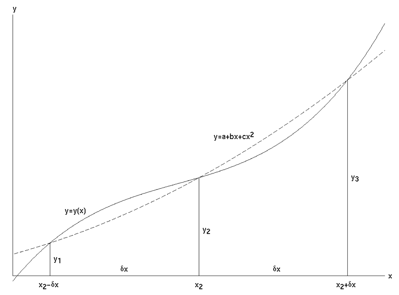
$\text{FIGURE I.1}$ Simpson's Rule gives us the area under the parabola (dashed curve) that passes through three points on the curve $y =y(x)$. This is approximately equal to the area under $y = y(x)$.

the function at $x_2 - δ_x, \ x_2$ and $x_2 + δ_x$, and $y = a + bx + cx^2$ is the parabola passing through the points $(x_2 - δx, y_1)$, $(x_2, y_2)$ and $(x_2 + δx, y_3)$.

If the parabola is to pass through these three points, we must have

$$y_1 = a + b(x_2 - δx) + c(x_2 - δx)^2 \label{1.2.1}$$

$$y_2 = a + bx + cx^2 \label{1.2.2}$$

$$y_3 = a + b(x_2 + δx) + c(x_2 + δx)^2 \label{1.2.3}$$

We can solve these Equations to find the values of $a$, $b$ and $c$. These are

$$a=y_2 - \frac{x_2(y_3-y_1)}{2δx} + \frac{x_2^2 (y_3 - 2y_2 + y_1)}{2(δx)^2} \label{1.2.4}$$

$$b = \frac{y_3 - y_1}{2δx} - \frac{x_2 (y_3 - 2y_2 + y_1)}{(δx)^2} \label{1.2.5}$$

$$c = \frac{y_3 - 2y_2 + y_1}{2(δx)^2} \label{1.2.6}$$

Now the area under the parabola (which is taken to be approximately the area under $y(x)$) is

$$\int_{x_2-δx}^{x_2+δx} \left( a+bx + cx^2 \right) dx = 2 \left[ a+bx_2 + cx_2^2 + \frac{1}{3} c (δx)^2 \right] δx \label{1.2.7}$$

On substituting the values of $a$, $b$ and $c$, we obtain for the area under the parabola

$$\frac{1}{3} (y_1 + 4y_2 + y_3 ) δx \label{1.2.8}$$

and this is the formula known as Simpson's Rule.

For an example, let us evaluate $\int_0^{\pi/2} \sin xdx$.

We shall evaluate the function at the lower and upper limits and halfway between. Thus

$$\begin{array}{l l} x= 0, & y=0 \\ x = \pi/4, & y=1/\sqrt{2} \\ x = \pi/2, & y=1 \\ \nonumber \end{array}$$

The interval between consecutive values of $x$ is $δx = \pi/4$.

Hence Simpson's Rule gives for the area

$$\frac{1}{3} \left( 0 + \frac{4}{\sqrt{2}}+ 1 \right) \frac{\pi}{4}\nonumber$$

which, to three significant figures, is $1.00$. Graphs of $\sin x$ and $a + bx + cx^2$ are shown in figure $\text{I.2a}$. The values of $a$, $b$ and $c$, obtained from the formulas above, are

$$a=0, \quad b = \frac{\sqrt{32}-2}{\pi}, \quad c = \frac{8-\sqrt{128}}{\pi^2} \nonumber$$

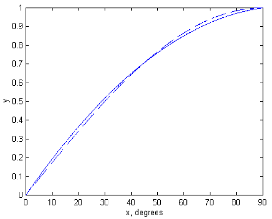
$\text{FIGURE I.2a}$

The result we have just obtained is quite spectacular, and we are not always so lucky. Not all functions can be approximated so well by a parabola. But of course the interval $δx = \pi/4$ was ridiculously coarse. In practice we subdivide the interval into numerous very small intervals. For example, consider the integral

$$\int_0^{\pi/4} \cos^{\frac{3}{2}} 2x \sin x\,dx .\nonumber$$

Let us subdivide the interval $0$ to $\pi/4$ into ten intervals of width $\pi /40$ each. We shall evaluate the function at the end points and the nine points between, thus:

$$\begin{array}{c c} x & \cos^{\frac{3}{2}} x \sin xdx \\ 0 & y_1 = 0.000 \ 000 \ 000 \\ \pi/40 & y_2 = 0.077 \ 014 \ 622 \\ 2\pi/40 & y_3 = 0.145 \ 091 \ 486 \\ 3\pi/40 & y_4 = 0.196 \ 339 \ 002 \\ 4\pi / 40 & y_5 = 0.224 \ 863 \ 430 \\ 5\pi / 40 & y_6 = 0.227 \ 544 \ 930 \\ 6\pi/40 & y_7 = 0.204 \ 585 \ 473 \\ 7\pi/40 & y_8 = 0.159 \ 828 \ 877 \\ 8\pi/40 & y_9 = 0.100 \ 969 \ 971 \\ 9\pi/40 & y_{10} = 0.040 \ 183 \ 066 \\ 10\pi/40 & y_{11} = 0.000 \ 000 \ 000 \\ \nonumber \end{array}$$

The integral from $0$ to $2\pi /40$ is $\frac{1}{3} (y_1 + 4y_2 + y_3) δx, \ δx$ being the interval $\pi/40$. The integral from $3\pi/40$ to $4\pi/40$ is $\frac{1}{3} ( y_3 +4y_4 +y_5 ) δx$. And so on, until we reach the integral from $8\pi/40$ to $10\pi/40$. When we add all of these up, we obtain for the integral from $0$ to $\pi /4$,

$$\frac{1}{3} \left( y_1 + 4y_2 + 2y_3 + 4y_4 + 2y_5 + ... ... + 4y_{10} + y_{11} \right) δx \nonumber$$

$$=\frac{1}{3} [ y_1 + y_{11} + (y_2 + y_4 + y_6 + y_8 + y_{10} ) + 2(y_3 + y_5 + y_7 + y_9 ) ] δx, \nonumber$$

which comes to $0.108 \ 768 \ 816$.

We see that the calculation is rather quick, and it is easily programmable (try it!). But how good is the answer? Is it good to three significant figures? Four? Five?

Since it is fairly easy to program the procedure for a computer, my practice is to subdivide the interval successively into $10$, $100$, $1000$ subintervals, and see whether the result converges. In the present example, with $N$ subintervals, I found the following results:

$$\begin{array}{r c} N & \text{integral} \\ \\ 10 & 0.108 \ 768 \ 816 \\ 100 & 0.108 \ 709 \ 621 \\ 1000 & 0.108 \ 709 \ 466 \\ 10000 & 0.108 \ 709 \ 465 \\ \nonumber \end{array}$$

This shows that, even with a course division into ten intervals, a fairly good result is obtained, but you do have to work for more significant figures. I was using a mainframe computer when I did the calculation with $10000$ intervals, and the answer was displayed on my screen in what I would estimate was about one fifth of a second.

There are two more lessons to be learned from this example. One is that sometimes a change of variable will make things very much faster. For example, if one makes one of the (fairly obvious?) trial substitutions $y = \cos x$, $y = \cos 2x$ or $y^2 = \cos 2x$, the integral becomes

$$\int_{1/\sqrt{2}}^1 (2y^2 - 1 )^{3/2} dy, \quad \int_0^1 \sqrt{\frac{y^3}{8(1+y)}} dy \quad \text{or} \quad \int_0^1 \frac{y^4}{\sqrt{2(1+y^2)}}dy. \nonumber$$

Not only is it very much faster to calculate any of these integrands than the original trigonometric expression, but I found the answer $0.108 \ 709 \ 465$ by Simpson's rule on the third of these with only $100$ intervals rather than $10,000$, the answer appearing on the screen apparently instantaneously. (The first two required a few more intervals.)

To gain about one fifth of a second may appear to be of small moment, but in truth the computation went faster by a factor of several hundred. One sometimes hears of very large computations involving massive amounts of data requiring overnight computer runs of eight hours or so. If the programming speed and efficiency could be increased by a factor of a few hundred, as in this example, the entire computation could be completed in less than a minute.

The other lesson to be learned is that the integral does, after all, have an explicit algebraic form. You should try to find it, not only for integration practice, but to convince yourself that there are indeed occasions when a numerical solution can be found faster than an analytic one! The answer, by the way, is $\frac{\sqrt{18}\ln(1+\sqrt{2}) - 2}{16}.$

You might now like to perform the following integration numerically, either by hand calculator or by computer.

$$\int_0^2 \frac{x^2 dx}{\sqrt{2-x}} \nonumber$$

At first glance, this may look like just another routine exercise, but you will very soon find a small difficulty and wonder what to do about it. The difficulty is that, at the upper limit of integration, the integrand becomes infinite. This sort of difficulty, which is not infrequent, can often be overcome by means of a change of variable. For example, let $x = 2 \sin^2 \theta$, and the integral becomes

$$8 \sqrt{2} \int_0^{\pi/2} \sin^5 \theta d \theta \nonumber$$

and the difficulty has gone. The reader should try to integrate this numerically by Simpson's rule, though it may also be noted that it has an exact analytic answer, namely $\sqrt{8192}/15$.

Here is another example. It can be shown that the period of oscillation of a simple pendulum of length $l$ swinging through $90^\circ$ on either side of the vertical is

$$P = \sqrt{\frac{8l}{g}} \int_0^{\pi/2} \sqrt{\sec \theta} d\theta . \nonumber$$

As in the previous example, the integrand becomes infinite at the upper limit. I leave it to the reader to find a suitable change of variable such that the integrand is finite at both limits, and then to integrate it numerically. (If you give up, see Section 1.13.) Unlike the last example, this one has no simple analytic solution in terms of elementary functions. It can be written in terms of special functions (elliptic integrals) but they have to be evaluated numerically in any case, so that is of little help. I make the answer

$$P = 2.3607 \pi \sqrt{\frac{l}{g}} . \nonumber$$

For another example, consider

$$\int_0^\infty \frac{dx}{x^5 \left( e^{1/x} - 1\right)}\nonumber$$

This integral occurs in the theory of blackbody radiation. To help you to visualize the integrand, it and its first derivative are zero at $x = 0$ and $x = \infty$ and it reaches a maximum value of $21.201435$ at $x = 0.201405$. The difficulty this time is the infinite upper limit. But, as in the previous two examples, we can overcome the difficulty by making a change of variable. For example, if we let $x = \tan \theta$, the integral becomes

$$\int_0^{\pi/2} \frac{c^3 \left(c^2 + 1 \right) d\theta}{e^c - 1}, \text{where } c=\cot \theta = 1/x. \nonumber$$

The integrand is zero at both limits and is easily calculable between, and the value of the integral can now be calculated by Simpson's rule in a straightforward way. It also has an exact analytic solution, namely $\pi^4 /15$, though it is hard to say whether it is easier to arrive at this by analysis or by numerical integration.

Here’s another:

$$\int_0^\infty \frac{x^2 dx}{(x^2+9)(x^2+4)^2} \nonumber$$

The immediate difficulty is the infinite upper limit, but that is easily dealt with by making a change of variable: $x = \tan \theta$. The integral then becomes

$$\int_{\theta=0}^{\pi/2} \frac{t(t+1)d\theta}{(t+9)(t+4)^2} \nonumber$$

in which $t = \tan^2 \theta$. The upper limit is now finite, and the integrand is easy to compute - except, perhaps, at the upper limit. However, after some initial hesitation the reader will probably agree that the integrand is zero at the upper limit. The integrand looks like this:

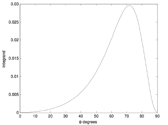
It reaches a maximum of $0.029 \ 5917$ at $\theta = 71^\circ .789 \ 962$. Simpson’s rule easily gave me an answer of $0.015 \ 708$. The integral has an analytic solution (try it) of $\pi/200$.

There are, of course, methods of numerical integration other than Simpson’s rule. I describe one here without proof. I call it “seven-point integration”. It may seem complicated, but once you have successfully programmed it for a computer, you can forget the details, and it is often even faster and more accurate than Simpson’s rule. You evaluate the function at $6n + 1$ points, where $n$ is an integer, so that there are $6n$ intervals. If, for example, $n = 4$, you evaluate the function at $25$ points, including the lower and upper limits of integration. The integral is then:

$$\int_a^b f(x)dx = 0.3 \times (\Sigma_1 + 2 \Sigma_2 + 5 \Sigma_3 + 6\Sigma_4)δx, \label{1.2.9}$$

where $δx$ is the size of the interval, and

$$\Sigma_1 = f_1 + f_3 + f_5 + f_9 + f_{11} + f_{15} + f_{17} + f_{21} + f_{23} + f_{25} , \label{1.2.10}$$

$$\Sigma_2 = f_7 + f_{13} + f_{19} , \label{1.2.11}$$

$$\Sigma_3 = f_2 + f_6 + f_8 + f_{12} + f_{14} + f_{18} + f_{20} + f_{24} \label{1.2.12}$$

and $$\Sigma_4 = f_4 + f_{10} + f_{16} + f_{22} . \label{1.2.13}$$

Here, of course, $f_1 = f(a)$ and $f_{25} = f(b)$. You can try this on the functions we have already integrated by Simpson’s rule, and see whether it is faster.

Let us try one last integration before moving to the next section. Let us try

$$\int_0^{10} \frac{1}{1+8x^3} dx . \nonumber$$

This can easily (!) be integrated analytically, and you might like to show that it is

$$\frac{1}{12} \ln \frac{147}{127} + \frac{1}{\sqrt{12}} \tan^{-1} \sqrt{507} + \frac{\pi}{\sqrt{432}} = 0.6039748 . \nonumber$$

However, our purpose in this section is to learn some skills of numerical integration. Using Simpson’s rule, I obtained the above answer to seven decimal places with $544$ intervals. With seven-point integration, however, I used only $162$ intervals to achieve the same precision, a reduction of $70%$. Either way, the calculation on a fast computer was almost instantaneous. However, had it been a really lengthy integration, the greater efficiency of the seven point integration might have saved hours. It is also worth noting that $x \times x \times x$ is faster to compute than $x^3$. Also, if we make the substitution y = 2x, the integral becomes

$$\int_0^{20} \frac{0.5}{1+y^3} dy . \nonumber$$

This reduces the number of multiplications to be done from $489$ to $326$ – i.e. a further reduction of one third. But we have still not done the best we could do. Let us look at the function $\frac{0.5}{1+y^3}$, in figure I.2b:

$\text{FIGURE I2b}$

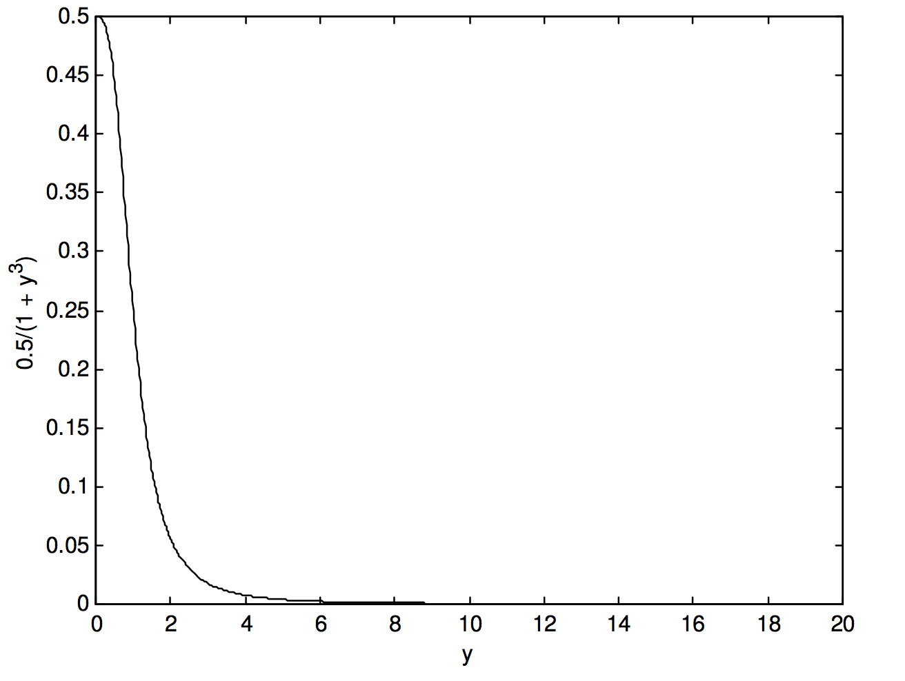
We see that beyond $y = 6$, our efforts have been largely wasted. We don’t need such fine intervals of integration. I find that I can obtain the same level of precision − i.e. an answer of $0.6039748$ − using 48 intervals from $y = 0$ to $6$ and $24$ intervals from $y = 6$ to $20$. Thus, by various means we have reduced the number of times that the function had to be evaluated from our original $545$ to $72$, as well as reducing the number of multiplications each time by a third, a reduction of computing time by $91%$. This last example shows that it often advantageous to use fine intervals of integration only when the function is rapidly changing (i.e. has a large slope), and to revert to coarser intervals where the function is changing only slowly.

The Gaussian quadrature method of numerical integration is described in Sections 1.15 and 1.16.