1.10: 1.10- Besselian Interpolation

In the days before the widespread use of high-speed computers, extensive use was commonly made of printed tables of the common mathematical functions. For example, a table of the Bessel function $J_0 (x)$ would indicate

$$J_0 (1.7) = 0.397 \ 984 \ 859 \nonumber$$

$$J_0(1.8) = 0.339 \ 986 \ 411 \nonumber$$

If one wanted the Bessel function for $x = 1.762$, one would have to interpolate between the tabulated values.

Today it would be easier simply to calculate the Bessel function for any particular desired value of the argument $x$, and there is less need today for printed tables or to know how to interpolate. Indeed, most computing systems today have internal routines that will enable one to calculate the commoner functions such as Bessel functions even if one has only a hazy notion of what a Bessel function is.

The need has not entirely passed, however. For example, in orbital calculations, we often need the geocentric coordinates of the Sun. These are not trivial for the nonspecialist to compute, and it may be easier to look them up in The Astronomical Almanac, where it is tabulated for every day of the year, such as, for example, July 14 and July 15. But, if one needs $y$ for July 14.395, how does one interpolate?

In an ideal world, a tabulated function would be tabulated at sufficiently fine intervals so that linear interpolation between two tabulated values would be adequate to return the function to the same number of significant figures as the tabulated points. The world is not perfect, however, and to achieve such perfection, the tabulation interval would have to change as the function changed more or less rapidly. We need to know, therefore, how to do nonlinear interpolation.

Suppose a function $y(x)$ is tabulated at $x = x_1$ and $x = x_2$, the interval $x_2 − x_1$ being $δx$. If one wishes to find the value of $y$ at $x + \theta δx$, linear interpolation gives

$$y(x_1 + \theta \Delta x) = y_1 + \theta (y_2 - y_1) = \theta y_2 + (1-\theta) y_1 , \label{1.10.1} \tag{1.10.1}$$

where $y_1 = y(x_1)$ and $y_2 = y(x_2)$. Here it is assumed that is a fraction between $0$ and $1$; if $\theta$ is outside this range (that is negative, or greater than $1$) we are extrapolating, not interpolating, and that is always a dangerous thing to do.

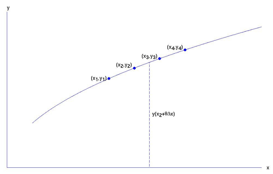
Let us now look at the situation where linear interpolation is not good enough. Suppose that a function $y(x)$ is tabulated for four points $x_1, \ x_2, \ x_3, \ x_4$ of the argument $x$, the corresponding values of the function being $y_1, \ y_2, \ y_3, \ y_4$. We wish to evaluate $y$ for $x = x_2 + \theta δx$, where $δx$ is the interval $x_2 - x_1$ or $x_3 - x_2$ or $x_4 - x_3$. The situation is illustrated in figure $\text{I.6A}$.

A possible approach would be to fit a polynomial to the four adjacent points:

$$y = a + bx + cx^2 + dx^3 .$$

We write down this Equation for the four adjacent tabulated points and solve for the coefficients, and hence we can evaluate the function for any value of $x$ that we like in the interval between $x_1$ and $x_4$. Unfortunately, this might well involve more computational effort than evaluating the original function itself.

$\text{FIGURE I.6A}$

The problem has been solved in a convenient fashion in terms of finite difference calculus, the logical development of which would involve an additional substantial chapter beyond the intended scope of this book. I therefore just provide the method only, without proof.

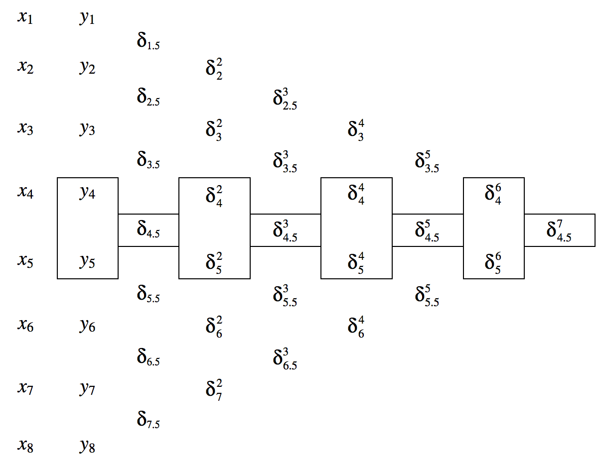
The essence of the method is to set up a table of differences as illustrated below. The first two columns are $x$ and $y$. The entries in the remaining columns are the differences between the two entries in the column immediately to the left. Thus, for example, $δ_{4.5} = y_5 - y_4$, $δ_4^2 = δ_{4.5} - δ_{3.5}$, etc.

Let us suppose that we want to find $y$ for a value of $x$ that is a fraction $\theta$ of the way from $x_4$ to $x_5$. Bessel's interpolation formula is then

$$y(x) = \frac{1}{2} (y_4 + y_5) + B_1 δ_{4.5} + B_2 ( δ_4^2 + δ_5^2) + B_3 δ_{4.5}^3 + B_4 (δ_4^4 + δ_5^4) + ... \label{1.10.3} \tag{1.10.3}$$

Here the $B_n$ are the Besselian interpolation coefficients, and the successive terms in parentheses in the expansion are the sums of the numbers in the boxes in the table.

The Besselian coefficients are

$$B_n (\theta) = \frac{1}{2} \begin{pmatrix} \theta + \frac{1}{2}n - 1 \\ n \end{pmatrix} \quad \text{if n is even,} \label{1.10.4} \tag{1.10.4}$$

and $$B_n (\theta) = \frac{\theta - \frac{1}{2}}{n} \begin{pmatrix} \theta + \frac{1}{2}n - \frac{3}{2} \\ n-1 \end{pmatrix} \quad \text{if n is odd.} \label{1.10.5} \tag{1.10.5}$$

The notation $\begin{pmatrix} m \\ n \end{pmatrix}$ means the coefficient of x m in the binomial expansion of $(1 + x)^n$.

Explicitly,

$$B_1 = \theta - \frac{1}{2} \label{1.10.6} \tag{1.10.6}$$

$$B_2 = \frac{1}{2} \theta ( \theta - 1 ) / 2! = \theta (\theta - 1) / 4 \label{1.10.7} \tag{1.10.7}$$

$$B_3 = (\theta - \frac{1}{2}) \theta ( \theta - 1) / 3! = \theta (0.5 + \theta (-1.5 + \theta ))/6 \label{1.10.8} \tag{1.10.8}$$

$$B_4 = \frac{1}{2} ( \theta + 1) \theta ( \theta - 1) ( \theta - 2) / 4 ! = \theta ( 2 + \theta ( -1 + \theta ( -2 + \theta ))) / 48 \label{1.10.0} \tag{1.10.9}$$

$$B_5 = (\theta - \frac{1}{2} ) ( \theta + 1) \theta ( \theta - 1) (\theta - 2) / 5 ! = \theta ( -1 + \theta ( 2.5 + \theta^2 (-2.5 + \theta )))/120 \label{1.10.10} \tag{1.10.10}$$

The reader should convince him- or herself that the interpolation formula taken as far as $B_1$ is merely linear interpolation. Addition of successively higher terms effectively fits a curve to more and more points around the desired value and more and more accurately reflects the actual change of $y$ with $x$.

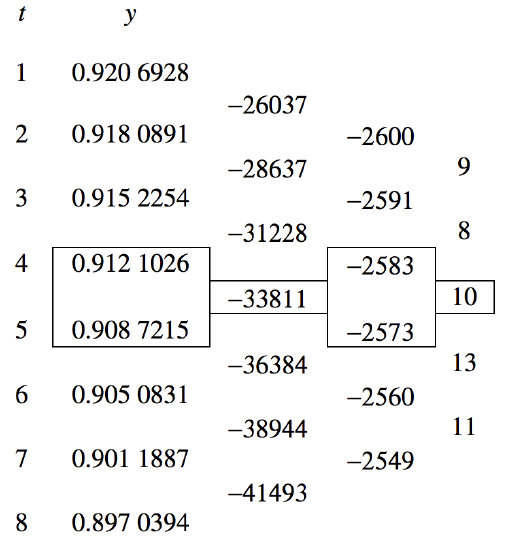
The above table is taken from The Astronomical Almanac for 1997, and it shows the $y$-coordinate of the Sun for eight consecutive days in July. The first three difference columns are tabulated, and it is clear that further difference columns are unwarranted.

If we want to find the value of $y$, for example, for July 4.746, we have $\theta = 0.746$ and the first three Bessel coefficients are

$$\begin{array}{c c l} B_1 & = & +0.246 \\ B_2 & = & -0.047 \ 371 \\ B_3 & = & -0.007 \ 768 \ 844 \\ \nonumber \end{array}$$

The reader can verify the following calculations for $y$ from the sum of the first 2, 3 and 4 terms of the Besselian interpolation series formula. The sum of the first two terms is the result of linear interpolation.

Sum of the first 2 terms, $y = 0.909 \ 580 \ 299$
Sum of the first 3 terms, $y = 0.909 \ 604 \ 723$
Sum of the first 4 terms, $y = 0.909 \ 604 \ 715$

Provided the table is not tabulated at inappropriately coarse intervals, one need rarely go past the third Bessel coefficient. In that case an alternative and equivalent interpolation formula (for $t = t_4 + \theta \Delta t)$, which avoids having to construct a difference table, is

$$\begin{array}{c c l} y(t_4 + \theta \Delta t) & = & -\frac{1}{6} \theta [ (2 - \theta ( 3- \theta )) y_3 + (1 - \theta ) y_6 ] \\ & & + \frac{1}{2} [(2 + \theta(-1 + \theta ( -2 + \theta))) y_4 + \theta ( 2 + \theta (1 - \theta)) y_5 ]. \end{array}$$

Readers should check that this gives the same answer, at the same time noting that the nested parentheses make the calculation very rapid and they are easy to program on either a calculator or a computer.

Exercise $\PageIndex{1}$: Bessel Coefficients

From the following table, construct a difference table up to fourth differences. Calculate the first four Bessel coefficients for $\theta = 0.73$. Hence calculate the value of $y$ for $x = 0.273$.

$$\begin{array}{c c} x & y \\ 0.0 & + 0.381300 \\ 0.1 & + 0.285603 \\ 0.2 & + 0.190 092 \\ 0.3 & + 0.096327 \\ 0.4 & + 0.008 268 \\ 0.5 & - 0.067 725 \\ \end{array}$$

Answers

• $B_1 = +0.23$
• $B_2 - - 0.049275$
• $B_3 = -7.5555 \times 10^{-3}$
• $B_4 = +9.021841875 \times 10^{-3}$
• $y = 0.121289738$

Note: the table was calculated from a formula, and the interpolated answer is correct to nine significant figures.

Exercise $\PageIndex{2}$: Linear Interpolation vs. Besselian Interpolation

From the following table of $\sin x$, use linear interpolation and Besselian interpolation to estimate $\sin 51^\circ$ to three significant figures.

$$\begin{array}{c c} x^\circ & \sin x \\ \\ 0 & 0.0 \\ 30 & 0.5 \\ 60 & \sqrt{3}/2 - 0.86603 \\ 90 & 1.0 \\ \end{array}$$

Answers

• By linear interpolation, $\sin 51^\circ = 0.634.$
• By Besselian interpolation, $\sin 51^\circ = 0.776.$

The correct value is 0.777. You should be impressed – but there is more on interpolation to come, in Section 1.11.