1.9: Nonlinear Simultaneous Equations

We consider two simultaneous Equations of the form

\[f(x, \ y) = 0, \label{1.9.1}\]

\[g(x, \ y) = 0 \label{1.9.2}\]

in which the Equations are not linear.

As an example, let us solve the Equations

\[x^2 = \frac{a}{b-\cos y} \label{1.9.3}\]

\[x^3 - x^2 = \frac{a(y-\sin y \cos y)}{\sin^3 y} , \label{1.9.4}\]

in which \(a\) and \(b\) are constants whose values are assumed given in any particular case.

This may seem like an artificially contrived pair of Equations, but in fact a pair of Equations like this does appear in orbital theory.

We suggest here two methods of solving the Equations.

In the first, we note that in fact \(x\) can be eliminated from the two Equations to yield a single Equation in \(y\):

\[F(y) = aR^3 - R^2 - 2SR - S^2 = 0, \label{1.9.5}\]

where \[R = 1/(b-\cos y) \label{1.9.5a} \tag{1.9.5a}\]

and \[S = (y - \sin y \cos y ) / \sin^3 y . \label{1.9.5b} \tag{1.9.5b}\]

This can be solved by the usual Newton-Raphson method, which is repeated application of \(y = y − F / F^\prime\). The derivative of \(F\) with respect to \(y\) is

\[F^\prime = 3aR^2 R^\prime - 2RR^\prime - 2(S^\prime R + SR^\prime) - 2SS^\prime \label{1.9.6}\]

where \[R^\prime = -\frac{\sin y}{(b-\cos y)^2} \label{1.9.6a} \tag{1.9.6a}\]

and \[S^\prime = \frac{\sin y (1 - \cos 2y ) - 3\cos y (y- \frac{1}{2} \sin 2y)}{\sin^4 y} \label{1.9.6b} \tag{1.9.6b}\]

In spite of what might appear at first glance to be some quite complicated Equations, it will be found that the Newton-Raphson process, \(y = y − F / F^\prime\), is quite straightforward to program, although, for computational purposes, \(F\) and \(F^\prime\) are better written as

\[F = -S^2 + R(-2S + R (-1 + aR)) , \label{1.9.7a} \tag{1.9.7a}\]

and

\[F^\prime = 3aR^2 R^\prime - 2(R+S)(R^\prime + S^\prime ) \label{1.9.7b} \tag{1.9.7b}\]

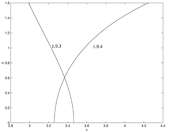
Let us look at a particular example, say with \(a = 36\) and \(b = 4\). We must of course, make a first guess. In the orbital application, described in Chapter 13, we suggest a first guess. In the present case, with \(a = 36\) and \(b = 4\), one way would be to plot graphs of Equations \(\ref{1.9.3}\) and \(\ref{1.9.4}\) and see where they intersect. We have done this in Figure 1.4, from which we see that y must be close to \(0.6\).

\(\text{FIGURE 1.4}\)
Equations \(\ref{1.9.3}\) and \(\ref{1.9.4}\) with \(a=36\) and \(b=4\).

With a first guess of \(y = 0.6\), convergence to \(y = 0.60292\) is reached in two iterations, and either of the two original Equations then gives \(x = 3.3666\).

We were lucky in this case in that we found we were able to eliminate one of the variables and so reduce the problem to a single Equation on one unknown. However, there will be occasions where elimination of one of the unknowns may be considerably more difficult or, in the case of two simultaneous transcendental Equations, impossible by algebraic means. The following iterative method, an extension of the Newton-Raphson technique, can nearly always be used. We describe it for two Equations in two unknowns, but it can easily be extended to \(n\) Equations in \(n\) unknowns.

The Equations to be solved are

\[f(x, \ y) = 0 \label{1.9.8} \tag{1.9.8}\]

\[g(x, \ y) = 0 . \label{1.9.9} \tag{1.9.9}\]

As with the solution of a single Equation, it is first necessary to guess at the solutions. This might be done in some cases by graphical methods. However, very often, as is common with the Newton-Raphson method, convergence is rapid even when the first guess is very wrong.

Suppose the initial guesses are \(x + h\), \(y + k\), where \(x\), \(y\) are the correct solutions, and \(h\) and \(k\) are the errors of our guess. From a first-order Taylor expansion (or from common sense, if the Taylor expansion is forgotten),

\[f(x+h, y+k) \approx f(x,y) + hf_x + kf_y . \label{1.9.10} \tag{1.9.10}\]

Here \(f_x\) and \(f_y\) are the partial derivatives and of course \(f(x, \ y) = 0\). The same considerations apply to the second Equation, so we arrive at the two linear Equations in the errors \(h\), \(k\):

\[f_x h + f_y k = f , \label{1.9.11} \tag{1.9.11}\]

\[g_x h + g_y k = g. \label{1.9.12} \tag{1.9.12}\]

These can be solved for \(h\) and \(k\):

\[h = \frac{g_y f - f_y g}{f_x g_y = f_y g_x}, \label{1.9.13} \tag{1.9.13}\]

\[k = \frac{f_x g - g_x f}{f_x g_y - f_y g_x}. \label{1.9.14} \tag{1.9.14}\]

These values of \(h\) and \(k\) are then subtracted from the first guess to obtain a better guess. The process is repeated until the changes in \(x\) and \(y\) are as small as desired for the particular application. It is easy to set up a computer program for solving any two Equations; all that will change from one pair of Equations to another are the definitions of the functions \(f\) and \(g\) and their partial derivatives.

In the case of our example, we have

\[f = x^2 - \frac{a}{b-\cos y} \label{1.9.15} \tag{1.9.15}\]

\[g = x^3 - x^2 - \frac{a(y-\sin y \cos y)}{\sin^3 y} \label{1.9.16} \tag{1.9.16}\]

\[f_x = 2x \tag{1.9.17} \label{1.9.17}\]

\[f_y = \frac{a\sin y}{(b- \cos y)^2} \label{1.9.18} \tag{1.9.18}\]

\[g_x = x(3x-2) \label{1.9.19} \tag{1.9.19}\]

\[g_y = \frac{a[3(y-\sin y \cos y) \cos y - 2\sin^3 y]}{\sin^4 y} \label{1.9.20} \tag{1.9.20}\]

In the particular case where \(a = 36\) and \(b = 4\), we can start with a first guess (from the graph - Figure I.4) of \(y = 0.6\) and hence \(x = 3.3\). Convergence to one part in a million is reached in three iterations, the solutions being \(x = 3.3666\), \(y = 0.60292\).

A simple application of these considerations arises if you have to solve a polynomial Equation \(f(z) = 0\), where there are no real roots, and all solutions for \(z\) are complex. You then merely write \(z = x + iy\) and substitute this in the polynomial Equation. Then equate the real and imaginary parts separately, to obtain two Equations of the form

\[R(x, \ y ) = 0 \label{1.9.21} \tag{1.9.21}\]

\[I(x, \ y ) = 0 \label{1.9.22} \tag{1.9.22}\]

and solve them for x and y. For example, find the roots of the Equation

\[z^4 - 5z + 6 = 0 . \label{1.9.23} \tag{1.9.23}\]

It will soon be found that we have to solve

\[R(x, \ y) = x^4 - 6x^2 y^2 + y^4 - 5x + 6 = 0 \label{1.9.24} \tag{1.9.24}\]

\[I(x, \ y) = 4x^3 - 4xy^2 - 5 = 0 \label{1.9.25} \tag{1.9.25}\]

It will have been observed that, in order to obtain the last Equation, we have divided through by \(y\), which is permissible, since we know \(z\) to be complex. We also note that \(y\) now occurs only as \(y^2\), so it will simplify things if we let \(y^2 = Y\), and then solve the Equations

\[f(x, Y) = x^4 - 6x^2 Y + Y^2 - 5x + 6 = 0 \label{1.9.26} \tag{1.9.26}\]

\[g(x,Y) = 4x^3 - 4xY - 5 = 0 \label{1.9.27} \tag{1.9.27}\]

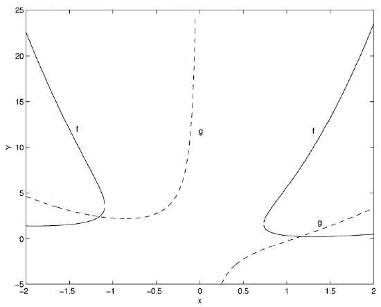
It is then easy to solve either of these for \(Y\) as a function of \(x\) and hence to graph the two functions (figure \(\text{I.5}\)):

\(\text{FIGURE I.5}\)

This enables us to make a first guess for the solutions, namely

\[x = -1.2, \quad Y = 2.4 \nonumber\]

and \[x= +1.2, \quad Y = 0.25818 \nonumber\]

We can then refine the solutions by the extended Newton-Raphson technique to obtain

\[x = -1.15697, \quad Y = 2.41899 \nonumber\]

\[x = +1.15697, \quad Y = 0.25818 \nonumber\]

so the four solutions to the original Equation are

\[z = -1.15697 \pm 1.55531i \nonumber\]

\[z = 1.15697 \pm 0.50812i \nonumber\]