3.2: Plane Triangles

This section is to serve as a brief reminder of how to solve a plane triangle. While there may be a temptation to pass rapidly over this section, it does contain a warning that will become even more pertinent in the section on spherical triangles.

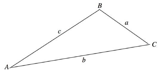
Conventionally, a plane triangle is described by its three angles \(A\), \(B\), \(C\) and three sides \(a\), \(b\), \(c\), with a being opposite to \(A\), \(b\) opposite to \(B\), and \(c\) opposite to \(C\). See figure \(\text{III.1}\).

\(\text{FIGURE III.1}\)

It is assumed that the reader is familiar with the sine and cosine formulas for the solution of the triangle:

\[\frac{a}{\sin A} = \frac{b}{\sin B} = \frac{c}{\sin C} \label{3.2.1} \tag{3.2.1}\]

and \[a^2 = b^2 + c^2 - 2bc \cos A , \label{3.2.2} \tag{3.2.2}\]

and understands that the art of solving a triangle involves recognition as to which formula is appropriate under which circumstances. Two quick examples - each with a warning - will suffice.

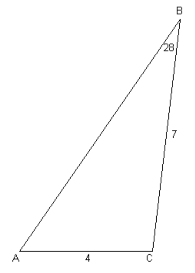
Example: A plane triangle has sides \(a = 7\) inches, \(b = 4\) inches and angle \(B = 28^\circ\). Find the angle \(A\).

\(\text{FIGURE III.2}\)

See figure \(\text{III.2}\)

We use the sine formula, to obtain

\(\sin A = \frac{7 \sin 28^\circ}{4} = 0.821575\)

\(A = 55^\circ 14^\prime .6\)

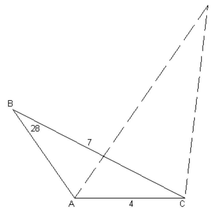
The pitfall is that there are two values of \(A\) between \(0^\circ\) and \(180^\circ\) that satisfy \(\sin A = 0.821575\), namely \(55^\circ \ 14^\prime.6\) and \(124^\circ \ 45^\prime.4\). Figure \(\text{III.3}\) shows that, given the original data, either of these is a valid solution.

\(\text{FIGURE III.3}\)

The lesson to be learned from this is that all inverse trigonometric functions \((\sin^{-1} , \cos^{-1} , \tan^{-1} )\) have two solutions between \(0^\circ\) and \(360^\circ\). The function \(\sin^{-1}\) is particularly troublesome since, for positive arguments, it has two solutions between \(0^\circ\) and \(180^\circ\). The reader must always be on guard for "quadrant problems" (i.e. determining which quadrant the desired solution belongs to) and is warned that, unless particular care is taken in programming calculators or computers, quadrant problems are among the most frequent problems in trigonometry, and especially in spherical astronomy.

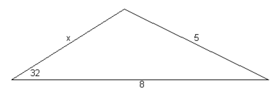
Example: Find \(x\) in the triangle illustrated in figure \(\text{III.4}\).

\(\text{FIGURE III.4}\)

Application of the cosine rule results in

\(25 = x^2 + 64 - 16x \cos 32^\circ\)

Solution of the quadratic Equation yields

\(x = 4.133 \ \text{or} \ 9.435\)

This illustrates that the problem of "two solutions" is not confined to angles alone. Figure \(\text{III.4}\) is drawn to scale for one of the solutions; the reader should draw the second solution to see how it is that two solutions are possible.

The reader is now invited to try the following "guaranteed all different" problems by hand calculator. Some may have two real solutions. Some may have none. The reader should draw the triangles accurately, especially those that have two solutions or no solutions. It is important to develop a clear geometric understanding of trigonometric problems, and not merely to rely on the automatic calculations of a machine. Developing these critical skills now will pay dividends in the more complex real problems encountered in celestial mechanics and orbital computation.

\(\text{PROBLEMS}\)

1. \(a = 6\ \ b = 4\ \ c = 7 \ C = ?\)

2. \(a= 5\ \ b = 3\ \ C = 43^\circ \ c = ?\)

3. \(a = 7\ \ b=9\ \ C = 110^\circ \ B=?\)

4. \( a = 4\ \ b=5\ \ A=29^\circ \ c = ? \)

5. \(a = 5\ \ b = 7\ \ A = 37^\circ \ B = ?\)

6. \(a = 8\ \ b=5\ \ A=54^\circ \ C=?\)

7. \(A=64^\circ \ B = 37^\circ \ a/c = ? \ b/c = ?\)

8. \(a = 3\ \ b = 8\ \ c = 4 \ C = ? \)

9. \(a = 4\ \ b=11\ \ A = 26^\circ \ c = ? \)

The reader is now further invited to write a computer program (in whatever language is most familiar) for solving each of the above problems for arbitrary values of the data. Lengths should be read in input and printed in output to four significant figures. Angles should be read in input and printed in output in degrees, minutes and tenths of a minute (e.g. \(47^\circ \ 12^\prime.9\)). Output should show two solutions if there are two, and should print "NO Solution" if there are none. This exercise will familiarize the reader with the manipulation of angles, especially inverse trigonometric functions in whatever computing language is used, and will be rewarded in future more advanced applications.

Solutions to problems.

1. \(C = 86^\circ 25^\prime.0\)
2. \(c=3.473\)
3. \(B=40^\circ 00^\prime.1\)
4. \(c=7.555 \text{ or } 1.191\)
5. \(B=57^\circ 24^\prime .6 \text{ or } 122^\circ 35^\prime .4\)
6. \(C=95^\circ 37^\prime .6 \text{ or } 23^\circ 37^\prime .6\)
7. \(a/c = 0.9165 \ b/c = 0.6131\)
8. No real solution
9. No real solution

The area of a plane triangle is \(\frac{1}{2} × \text{base} × \text{height}\), and it is easy to see from this that

\[\text{Area} = \frac{1}{2} bc \sin A = \frac{1}{2} ca \sin B = \frac{1}{2} ab \sin C \label{3.2.3} \tag{3.2.3}\]

By making use \(\sin^2 A = 1 - \cos^2 A\) and \(\cos A = \left( b^2 + c^2 - a^2 \right)/(2bc)\), we can express this entirely in terms of the lengths of the sides:

\[\text{Area} = \sqrt{s(s-a)(s-b)(s-c),} \label{3.2.4} \tag{3.2.4}\]

where \(s\) is the semi-perimeter \(\frac{1}{2}(a+b+c)\).