6.11: Solutions

6.11.1

I think the first thing that I would do, would be to convert the coordinates to degrees and decimals (or maybe even radians and decimals, though I do it below in degrees and decimals):

Antares: $α = 247.375 \quad δ = -26.433$
Deneb $α = 309.400 \quad δ = +45.283$

We already did a similar problem in Chapter 3, Section 3.5, Example 2, so I shan’t do it again. I make the answer:

One pole: $α = 11^\text{h} 47^\text{m} .3 \quad δ = + 56^\circ 11^\prime$
The other pole: $α = 23^\text{h} 47^\text{m} .3 \quad δ = + 123^\circ 49^\prime$

6.11.2

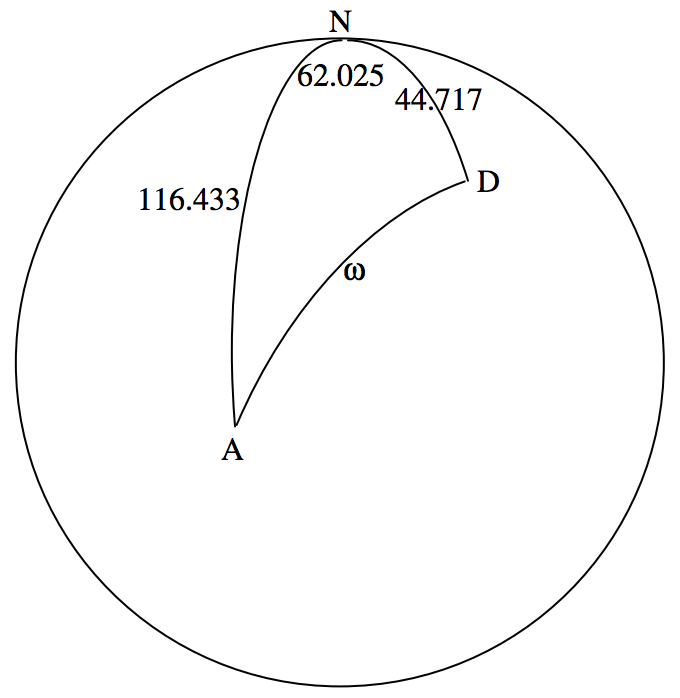
I have drawn the North Celestial Pole $\text{N}$, and the colures from $\text{N}$ to Antares ($\text{A}$) and to Deneb ($\text{D}$), together with their north polar distances in degrees. I have also marked the difference between their right ascensions, in degrees. We can immediately calculate, from the cosine rule for spherical triangles, Equation 3.5.2, the angular distance $ω$ between the two stars in the sky. I make it $ω = 91^\circ .190 \ 79$.

Now that we know the angle between the stars, we can use a plane triangle to calculate the distance between them:

I have marked Antares ($\text{A}$), Deneb ($\text{D}$) and us ($\text{O}$), and the distances from us to the two stars, in parsecs. (That’s the reciprocal of their parallaxes in arcsec.) I have also marked the angles, in degrees, between Antares and Deneb. We can now use the cosine rule for planes triangles, Equation 3.2.2, to find the distance $\text{AD}$. I make it 1011 parsecs.

A parsec is the distance at which an astronomical unit (approximately the radius of Earth’s orbit) would subtend an angle of one arcsecond. This also means, if you come to think of it, that the number of astronomical units in a parsec is equal to the number of arcseconds in a radian, which is $360 \times 3600 \div (2π) = 2.062648 \times 10^5$. The distance between the stars is therefore $1011 \times 2.062648 \times 10^5$ astronomical units. Multiply this by $1.495 \ 98 \times 10^8$, to get the distance in km. I make the distance $3.120 \times 10^{16} \ \text{km}$.

This would take light $1.040596 \times 10^8$ seconds to travel, or 3298 years, so the distance between the stars is 3298 light-years.

6.11.3

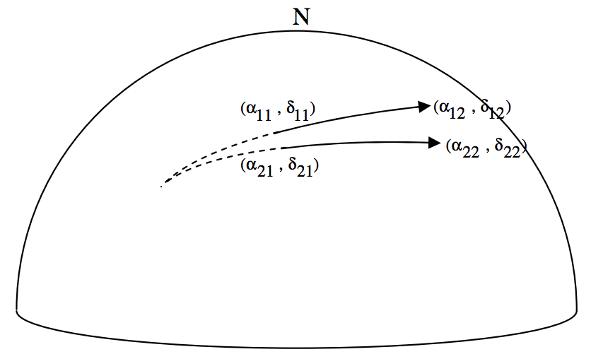
Let’s see if we can develop a formula for a general case. We’ll have the first meteor start at $(α_{11}, \ δ_{11})$ and finish at $(α_{12}, \ δ_{12})$. The second meteor starts at $(α_{21}, \ δ_{21})$ and finishes at $(α_{22}, \ δ_{22}$. We have to find the coordinates $(α, \ δ$ of the point from which the two meteors diverge.

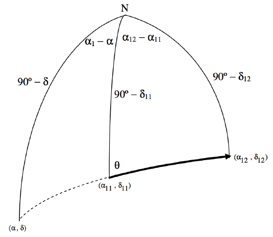
This is not a particularly easy problem – but is one that is obviously useful for meteor observers. I’ll just outline some suggestions here, and leave the reader to work out the details. I’ll draw below one of the meteors, and the radiant, and the North Celestial Pole:

Use the cotangent rule (Equation 3.5.5) on the righthand triangle to get an expression for $\cot θ$:

$$\sin δ_{11} \cos (α_{12} - α_{11}) = \cos δ_{11} \tan δ_{12} + \sin (α_{12} - α_{11}) \cot θ.$$

Equate these two expression for $\cot θ$ (i.e. eliminate $θ$ between the two Equations). This will give you a single Equation containing the two unknowns, $α$ and $δ$, everything else in the Equation being a known quantity. (This will be obvious if you are actually doing a numerical example.)

Now do the same thing for the second meteor, and you will get a second Equation in α and δ. In principle you are now home free, though there may be a bit of heavy algebra and trigonometry to go through before you finally get there.

I make the answer as follows:

$$\tan α = \frac{\cos α_{22} \tan δ_{22} - \cos α_{12} \tan δ_{12} + a_1 \sin α_{12} - a_2 \sin α_{22}}{\sin α_{12} \tan δ_{12} - \sin α_{22} \tan δ_{22} + a_1 \cos α_{12} - a_2 \cos α_{22}},$$

where $$a_1 = \frac{\tan δ_{11}}{\sin(α_{11} - α_{12})} - \frac{\tan δ_{12}}{\tan(α_{11} - α_{12})}$$

and $$a_2 = \frac{\tan δ_{21}}{\sin(α_{21} - α_{22})} - \frac{\tan δ_{22}}{\tan(α_{21} - α_{22})}$$

Then $$\tan δ = \cos (α - α_{12}) \tan δ_{12} + \sin (α - α_{12} ) [\csc (α_{11} - α_{12}) \tan δ_{11} - \cot (α_{11} - α_{12}) \tan δ_{12}]$$

or $$\tan δ = \cos (α - α_{22}) \tan δ_{22} + \sin (α - α_{22} ) [\csc (α_{21} - α_{22}) \tan δ_{21} - \cot (α_{21} - α_{22}) \tan δ_{22}].$$

Either of these two Equations for $\tan δ$ should give the same result. In the computer program I use for this calculation, I get it to calculate $\tan δ$ from both Equations, just as a check for mistakes.

This may look complicated, but all terms are just calculable numbers for any particular case. If the equinoctial colure gets in the way (as it did – deliberately – in the numerical example I gave), I suggest just add 24 hours to all right ascensions.

For the numerical example I gave, I make the coordinates of the radiant to be:

$$α = 22^\text{h} 01^\text{m}.3 \quad δ = - 00^\circ 37^\prime .$$