6: Blackbody Radiation

Theoretical quantities: blackbody radiation

Magnitudes are observed quantities; that is, in practice, optical astronomers typically

1. take pictures of stars
2. measure the apparent brightness of each star
3. convert the measurement to an instrumental magnitude
4. compare to the magnitudes in a standard catalog

As you can see, there are actually several steps involved in this procedure (and, if you try to do it yourself, you'll find that each of these steps has smaller steps within it). But the bottom line is that most optical measurements are differential: we compare one star in a frame to another star in the same frame, using magnitudes. For example, you might hear an astronomer mutter:

"Let's see ... my target object is about 2.4 magnitudes fainter than star A in the chart. Hmmmm. The USNO-A2.0 catalog lists a magnitude mR = 18.3 for star A, so that makes my target object magnitude mR = 20.7."

You will very rarely hear an astronomer talk about his measurements in terms of the physical quantities you might expect:

<Uncommon> "Ah, I detect a flux of 4.3 microwatts per square cm per sec from my target." </Uncommon>

Why not? If you were testing a set of light bulbs inside a lab, you'd surely measure some quantity like watts per square cm per second. So why do astronomers adopt this awkward scheme of differential measurement?

Exercise \(\PageIndex{1}\)

What's wrong with astronomers?

The answer is that astronomers aren't sitting inside a small laboratory room. Instead, they are sitting at the bottom of several miles of air, a mixture of several gases, dust and other contaminants, with layers at different heights and temperatures, all moving constantly. Oh, and their sources are ALSO moving relative to the air, so the path of light from any particular source samples a different column of air as time goes by.

Just as an example, take a look at these measurements of light from one particular star on July 27, 2001, at the RIT Observatory:

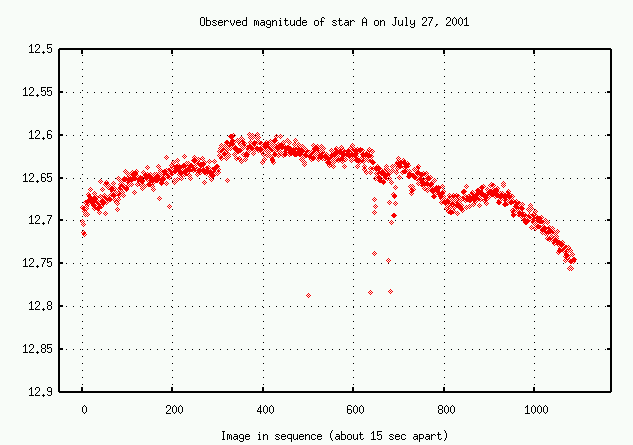
In fact, this star is one which we believe to be constant: the amount of light it produces doesn't change significantly over timescales of a few hours. All the changes in the observed signal you see above are due to the Earth's atmosphere. Bleah.

You can spend years learning about the nasty properties of real observing and data reduction. But that's really the subject of a different course.

In this course, we will spend most of our time considering the intrinsic, physical properties of stars. Of course, we must connect these physical properties to the measured quantities eventually. But let's take a little time to talk about light from a star in the theoretical sense. As a first approximation, we'll treat stars as perfect spheres of uniform composition and temperature, radiating as perfect blackbodies. So let's review the properties of blackbody radiation.

Blackbody Radiation

As a general rule, bodies give off radiation in a particular way that depends on their temperature. Consider a small patch of material at temperature \(T\). If this material is a perfect emitter (and absorber) of radiation, then the total amount of energy it emits per second, its luminosity \(L\) is

\[L=A \sigma T^{4}\]

where \(A\) is the area of the patch, \(σ\) is the Stefan-Boltzmann constant, and \(T\) is measured in Kelvin.

Clearly, this is a strong function of temperature. Increasing the temperature of a star even a little bit will increase its luminosity quite a bit.

Exercise \(\PageIndex{2}\)

If the temperature of a star increases by 10%, by what percent does its luminosity rise?

Estimate your own luminosity. Express the result in both ergs per second, and in watts.

To a decent approximation, stars are nearly blackbodies and nearly spheres. That means that the total luminosity of a star can be estimated from its radius \(R\) and temperature \(T\).

\[L=4 \pi R^{2} \sigma T^{4}\]

To measure the luminosity of a star, strictly speaking, we would have to collect every photon it emits by building a sphere completely enclosing it (a Dyson sphere). That's not possible. The quantity we can actually measure is the flux: the energy passing through some area during some time. In cgs, the units of flux are

\[\text{flux: ergs per square cm per second}\nonumber\]

The flux one measures from a star should decrease as one moves away from it, following the inverse square law. So, if we could measure the flux from a star, and we knew its distance, and we assume it emits radiation isotropically, we could calculate its luminosity.

Exercise \(\PageIndex{3}\)

On a clear day, the flux from the Sun at the Earth's surface is very roughly one million ergs/sq.cm/sec

What is the Sun's luminosity?

The spectrum of blackbody radiation

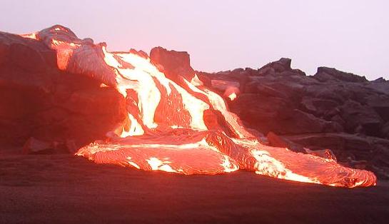
Not only do hot objects emit more energy from each unit area per unit time than cool objects, their radiation consists of a different mix of wavelengths, or frequencies, or energies. Qualitatively, lava at a temperature of 1000 Kelvin glows dull red:

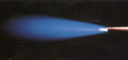
while an oxyacetylene flame at 3200 K is blueish-white:

Quantitatively speaking, the peak of an object's spectral energy distribution shifts to shorter wavelengths (or higher frequencies) as its temperature rises:

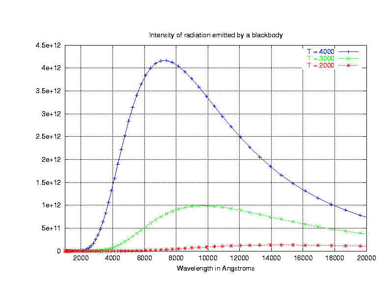
There is a simple connection between the temperature of a blackbody and the wavelength at which its intensity(*) reaches a peak:

(*) energy per unit area per unit time per unit wavelength

\[\lambda_{\text {peak }}=\frac{0.290 \text{ cm K}}{T}\]

At the turn of the twentieth century, German physicist Max Planck figured out a mathematical expression for the spectrum of radiation emitted from a blackbody, a (fictional) object which absorbs all incident radiation. This "Planck function" can be expressed in two ways:

• energy emitted per unit area per unit time per unit wavelength

\[B_{\lambda}(T)=\dfrac{2 h c^{2} / \lambda^{5}}{e^{h c / \lambda k T}-1}\]

• energy emitted per unit area per unit time per unit frequency

\[B_{\nu}(T)=\dfrac{2 h \nu^{3} / c^{2}}{e^{h \nu / k T}-1}\]

Be careful not to confuse these two very different expressions.

The units of \(B_{\nu}\) and \(B_{\lambda}\) are different, but you'll end up with the same thing -- flux, aka energy per unit area per unit time -- if you integrate either expression over some particular passband. For example, consider a filter which is a simple rectangle covering the entire visible region:

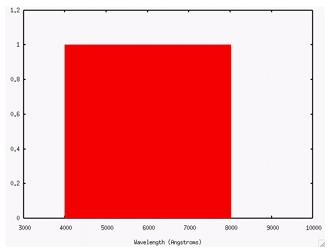
The limits of this filter are

• from 4E-5 cm to 8E-5 cm
• from 3.75E14 Hz to 7.5E14 Hz

So we should get the same total flux if we properly evaluate either of these integrals:

\[F=\int_{\lambda_{1}}^{\lambda_{2}} B_{\lambda}(T) d \lambda=\int_{\nu_{1}}^{\nu_{2}} B_{\nu}(T) d \nu\]

Can you evaluate these integrals to find the total flux through the passband? You can make an order-of-magnitude estimate by assuming that the spectrum of an object across the entire visible passband is constant, with the value appropriate for the middle of the passband (i.e. 6000 Angstroms = 6E-5 cm = 5E14 Hz).

Exercise \(\PageIndex{4}\)

Perform a very approximate calculation of the total flux through the above passband for T = 5600 K. Do you get the same result for an integration over wavelength as you do for an integration over frequency?

To do a good job, of course, you might use a numerical method like so:

• break the passband into many small intervals of wavelength or frequency
• evaluate the Planck function at the center of each interval
• assume that the spectrum has a constant value over the interval, and approximate the integral over this interval as the product
• add up all the products across the passband

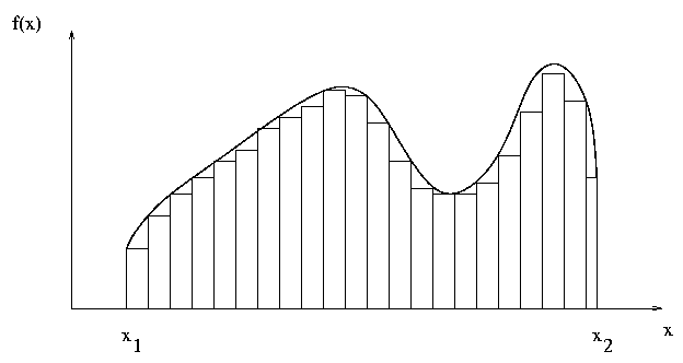
You can read a more detailed description of this simple numerical integration technique at some notes for the Computational Physics course.

Sources of astronomical spectra

Over the years, astronomers have measured and calibrated the spectra of a number of different types of celestial sources. If you need real spectra, in real units, consider looking at

• Spectrophotometric atlas of synthesis standard spectra by Pickles (1985). You can find the tabulated data in a nice searchable database thanks to Simbad.
• Stellar Spectrophotometric Atlas by Gunn and Stryker (1983), also available in an on-line version.
• A spectrophotometric atlas of galaxies by Kennicutt (1992). Once again, use SIMBAD to access an FTP archive.

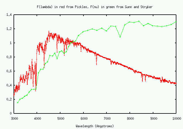
You must be very careful not to confuse the units used to measure flux. Here, for example, is the spectrum of a star like our Sun, a G2 dwarf, in units of flux per unit wavelength per square cm per second (the vertical scale is arbitrary). This is the usual way to report fluxes of stars, and is often called Flam for short.

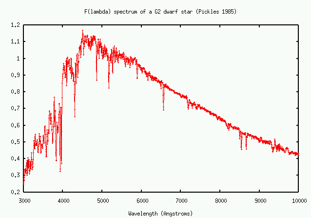
Compare the relative flux distributions for similar stars when plotted as F(lambda) versus as F(nu). The peaks occur at completely different locations!