
16: Removing the Tilt from a Visual Binary's Orbit
- Page ID
- 24358

\( \newcommand{\vecs}[1]{\overset { \scriptstyle \rightharpoonup} {\mathbf{#1}} } \)
\( \newcommand{\vecd}[1]{\overset{-\!-\!\rightharpoonup}{\vphantom{a}\smash {#1}}} \)
\( \newcommand{\dsum}{\displaystyle\sum\limits} \)
\( \newcommand{\dint}{\displaystyle\int\limits} \)
\( \newcommand{\dlim}{\displaystyle\lim\limits} \)
\( \newcommand{\id}{\mathrm{id}}\) \( \newcommand{\Span}{\mathrm{span}}\)
( \newcommand{\kernel}{\mathrm{null}\,}\) \( \newcommand{\range}{\mathrm{range}\,}\)
\( \newcommand{\RealPart}{\mathrm{Re}}\) \( \newcommand{\ImaginaryPart}{\mathrm{Im}}\)
\( \newcommand{\Argument}{\mathrm{Arg}}\) \( \newcommand{\norm}[1]{\| #1 \|}\)
\( \newcommand{\inner}[2]{\langle #1, #2 \rangle}\)
\( \newcommand{\Span}{\mathrm{span}}\)
\( \newcommand{\id}{\mathrm{id}}\)
\( \newcommand{\Span}{\mathrm{span}}\)
\( \newcommand{\kernel}{\mathrm{null}\,}\)
\( \newcommand{\range}{\mathrm{range}\,}\)
\( \newcommand{\RealPart}{\mathrm{Re}}\)
\( \newcommand{\ImaginaryPart}{\mathrm{Im}}\)
\( \newcommand{\Argument}{\mathrm{Arg}}\)
\( \newcommand{\norm}[1]{\| #1 \|}\)
\( \newcommand{\inner}[2]{\langle #1, #2 \rangle}\)
\( \newcommand{\Span}{\mathrm{span}}\) \( \newcommand{\AA}{\unicode[.8,0]{x212B}}\)
\( \newcommand{\vectorA}[1]{\vec{#1}} % arrow\)
\( \newcommand{\vectorAt}[1]{\vec{\text{#1}}} % arrow\)
\( \newcommand{\vectorB}[1]{\overset { \scriptstyle \rightharpoonup} {\mathbf{#1}} } \)
\( \newcommand{\vectorC}[1]{\textbf{#1}} \)
\( \newcommand{\vectorD}[1]{\overrightarrow{#1}} \)
\( \newcommand{\vectorDt}[1]{\overrightarrow{\text{#1}}} \)
\( \newcommand{\vectE}[1]{\overset{-\!-\!\rightharpoonup}{\vphantom{a}\smash{\mathbf {#1}}}} \)
\( \newcommand{\vecs}[1]{\overset { \scriptstyle \rightharpoonup} {\mathbf{#1}} } \)
\(\newcommand{\longvect}{\overrightarrow}\)
\( \newcommand{\vecd}[1]{\overset{-\!-\!\rightharpoonup}{\vphantom{a}\smash {#1}}} \)
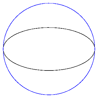
\(\newcommand{\avec}{\mathbf a}\) \(\newcommand{\bvec}{\mathbf b}\) \(\newcommand{\cvec}{\mathbf c}\) \(\newcommand{\dvec}{\mathbf d}\) \(\newcommand{\dtil}{\widetilde{\mathbf d}}\) \(\newcommand{\evec}{\mathbf e}\) \(\newcommand{\fvec}{\mathbf f}\) \(\newcommand{\nvec}{\mathbf n}\) \(\newcommand{\pvec}{\mathbf p}\) \(\newcommand{\qvec}{\mathbf q}\) \(\newcommand{\svec}{\mathbf s}\) \(\newcommand{\tvec}{\mathbf t}\) \(\newcommand{\uvec}{\mathbf u}\) \(\newcommand{\vvec}{\mathbf v}\) \(\newcommand{\wvec}{\mathbf w}\) \(\newcommand{\xvec}{\mathbf x}\) \(\newcommand{\yvec}{\mathbf y}\) \(\newcommand{\zvec}{\mathbf z}\) \(\newcommand{\rvec}{\mathbf r}\) \(\newcommand{\mvec}{\mathbf m}\) \(\newcommand{\zerovec}{\mathbf 0}\) \(\newcommand{\onevec}{\mathbf 1}\) \(\newcommand{\real}{\mathbb R}\) \(\newcommand{\twovec}[2]{\left[\begin{array}{r}#1 \\ #2 \end{array}\right]}\) \(\newcommand{\ctwovec}[2]{\left[\begin{array}{c}#1 \\ #2 \end{array}\right]}\) \(\newcommand{\threevec}[3]{\left[\begin{array}{r}#1 \\ #2 \\ #3 \end{array}\right]}\) \(\newcommand{\cthreevec}[3]{\left[\begin{array}{c}#1 \\ #2 \\ #3 \end{array}\right]}\) \(\newcommand{\fourvec}[4]{\left[\begin{array}{r}#1 \\ #2 \\ #3 \\ #4 \end{array}\right]}\) \(\newcommand{\cfourvec}[4]{\left[\begin{array}{c}#1 \\ #2 \\ #3 \\ #4 \end{array}\right]}\) \(\newcommand{\fivevec}[5]{\left[\begin{array}{r}#1 \\ #2 \\ #3 \\ #4 \\ #5 \\ \end{array}\right]}\) \(\newcommand{\cfivevec}[5]{\left[\begin{array}{c}#1 \\ #2 \\ #3 \\ #4 \\ #5 \\ \end{array}\right]}\) \(\newcommand{\mattwo}[4]{\left[\begin{array}{rr}#1 \amp #2 \\ #3 \amp #4 \\ \end{array}\right]}\) \(\newcommand{\laspan}[1]{\text{Span}\{#1\}}\) \(\newcommand{\bcal}{\cal B}\) \(\newcommand{\ccal}{\cal C}\) \(\newcommand{\scal}{\cal S}\) \(\newcommand{\wcal}{\cal W}\) \(\newcommand{\ecal}{\cal E}\) \(\newcommand{\coords}[2]{\left\{#1\right\}_{#2}}\) \(\newcommand{\gray}[1]{\color{gray}{#1}}\) \(\newcommand{\lgray}[1]{\color{lightgray}{#1}}\) \(\newcommand{\rank}{\operatorname{rank}}\) \(\newcommand{\row}{\text{Row}}\) \(\newcommand{\col}{\text{Col}}\) \(\renewcommand{\row}{\text{Row}}\) \(\newcommand{\nul}{\text{Nul}}\) \(\newcommand{\var}{\text{Var}}\) \(\newcommand{\corr}{\text{corr}}\) \(\newcommand{\len}[1]{\left|#1\right|}\) \(\newcommand{\bbar}{\overline{\bvec}}\) \(\newcommand{\bhat}{\widehat{\bvec}}\) \(\newcommand{\bperp}{\bvec^\perp}\) \(\newcommand{\xhat}{\widehat{\xvec}}\) \(\newcommand{\vhat}{\widehat{\vvec}}\) \(\newcommand{\uhat}{\widehat{\uvec}}\) \(\newcommand{\what}{\widehat{\wvec}}\) \(\newcommand{\Sighat}{\widehat{\Sigma}}\) \(\newcommand{\lt}{<}\) \(\newcommand{\gt}{>}\) \(\newcommand{\amp}{&}\) \(\definecolor{fillinmathshade}{gray}{0.9}\)In most cases, we will NOT see the orbit of a binary star face-on; and that means that we can't use the observed orbit to derive the mass of the system. Rats.
Remember that our plan is to use some form of Kepler's Third Law, like this:
\[P^{2}=\frac{4 \pi^{2}}{G M} a^{3} \nonumber \]
It's easy to measure the period \(\mathbf{P}\): we just wait for the secondary to complete one revolution around the primary. The more revolutions we observe, the more precisely we can measure \(\mathbf{P}\). But the semi-major axis a of the orbit is the problem. Unless we observe the orbit face-on, we won't see the true semi-major axis, and so we can't calculate the true total mass \(\mathbf{M}\) of the system.
So, the question is, given the observed orbit of the secondary around the primary, like this:
.jpg?revision=1)
how can we un-do the tilt and recover the semi-major axis \(\mathbf{a}\)? In addition, we might (for some purposes) want to determine exactly the axis of rotation and the amount of tilt, in order to recover the exact orientation of the real orbit in space.
This is a problem which has occupied astronomers for several centuries. There are many different approaches, some designed for particular circumstances, others more general. You can read about some of them in the references listed at the end of this lecture. I will show here one of the simplest methods, a graphical one which can be performed with nothing more than a ruler and pencil.
A little background: the eccentric circle
Given any ellipse, we can draw its eccentric circle by making the circle which
- has the same center as the ellipse
- has a radius equal to the semi-major axis of the ellipse
In other words, the eccentric circle circumscribes the given ellipse.
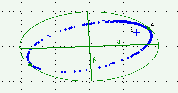
Now, if we start with an ellipse of \(\mathbf{e = 0.8}\) and its eccentric circle,
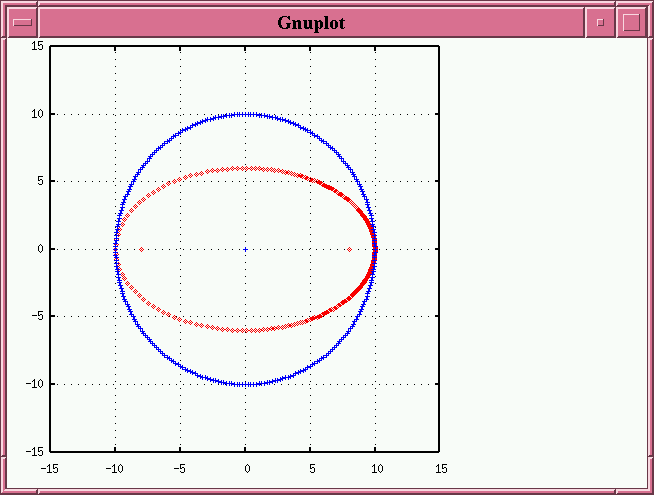
and subject them both to an arbitrary tilt (in this case \(\mathbf{i = 60} \textbf{ degrees}\)) around an arbitrary line of nodes (in this case tilted by \(\mathbf{ω = 30} \textbf{ degrees}\) relative to the true major axis), we create two new projected ellipses:
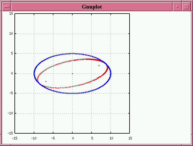
Note that the true foci of the orbit, shown as red dots, no longer appear along the principal axes of the projected ellipse. Also note several properties of the projected eccentric circle:
- its principal axes no longer line up with those of the projected orbital ellipse
- but it does still share its center with the projected orbital ellipse
- it touches the projected orbital ellipse at two points; the line connecting these points is parallel to the line of nodes
We call the projected version of the eccentric circle the auxiliary ellipse or eccentric ellipse which goes together with the projected orbital ellipse. We are going to use this auxiliary ellipse extensively in our work below.
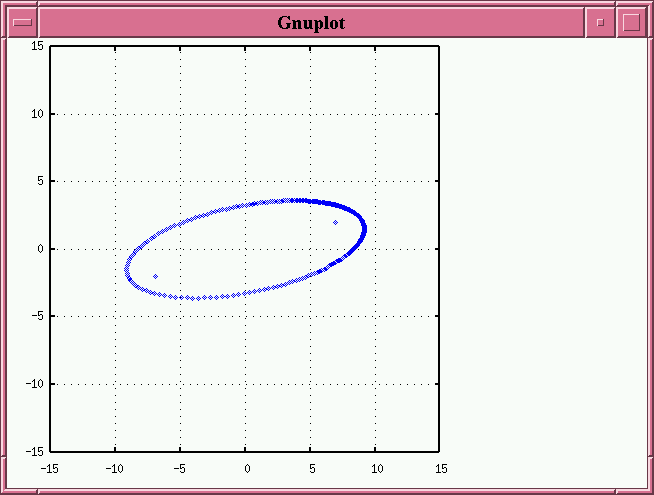
Step 1: sketch the apparent ellipse of the orbit
The first step is to plot the measurements of separation and position angle onto a piece of paper. They should define an ellipse.
Step 2: find projection of semi-major axis, and true eccentricity
Now, in the true orbit, we can draw a straight line connecting the center of the true ellipse, the location of the primary star (at one focus), and the perihelion of the secondary. This line lies along the major axis of the true orbit.
Yes, it would be more accurate to use the term "periastron", but I'd rather stick to familiar terms right now.
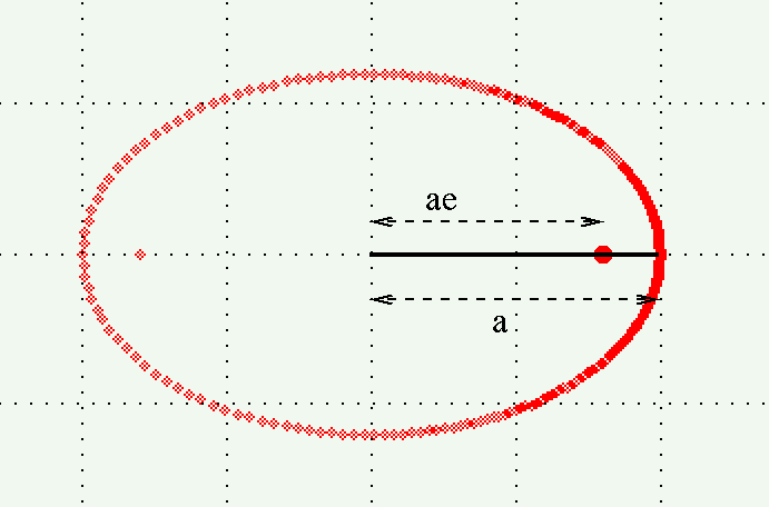
The ratio of (center-to-focus) to (center-to-perihelion) is simply
\[\frac{\text{(center-to-focus)}}{\text{(center-to-perihelion)}} = \frac{ae}{a} = e \nonumber \]
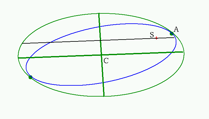
Now, these three points (center, focus, perihelion) remain colinear in the projected ellipse, and retain their relative positions. That means that we can draw this line on the projected ellipse:
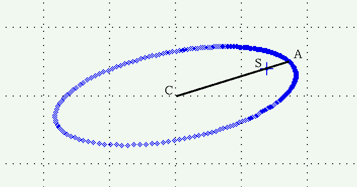
The ratio of the lengths CS to CA will again yield the eccentricity of the true ellipse, \(\mathbf{e}\).
That was easy! But the next bits involve more work...
Step 3a: calculate the constant k
We are going to draw the projection of the eccentric circle, that is, the auxiliary ellipse. It will take several steps.
The first thing to do is to calculate a constant value, \(\mathbf{k}\), based on the eccentricity \(\mathbf{e}\) of the true orbit.
\[k=\frac{1}{\sqrt{\left(1-e^{2}\right)}} \nonumber \]
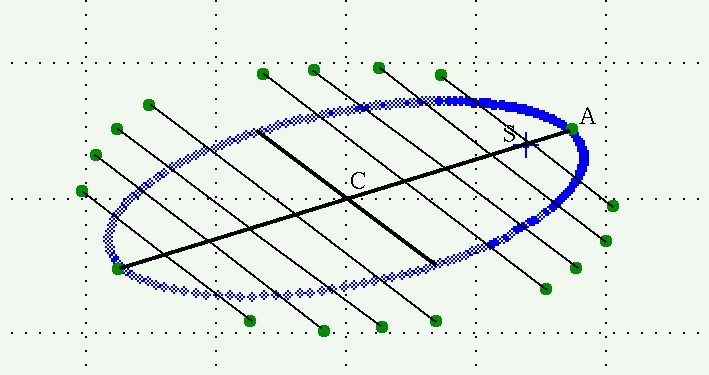
Step 3b: draw the projection of the minor axis of the orbit
Next, we draw the projection of the minor axis of the true orbit. Despite being projected, the major and minor axes of the true orbit remain conjugate. That means we can draw the minor axis like so:
- pick any chord on the observed ellipse which is parallel to the projected major axis
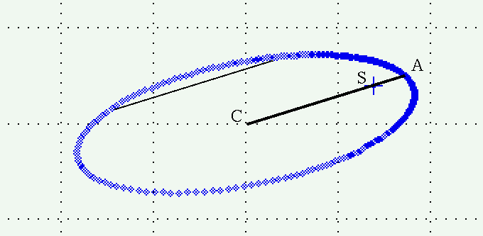
- bisect the chord
- extend the line running from the middle of the chord through the center of the observed ellipse so that it intersects the observed ellipse
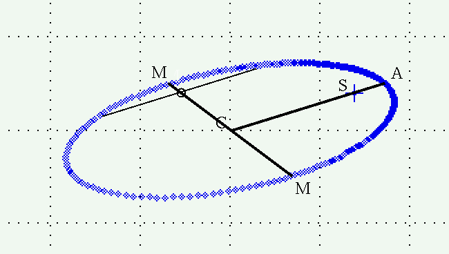
This line, marked M-M in the figure above, is the projection of the minor axis of the true orbit.
Step 3c: project outwards to define the auxiliary ellipse
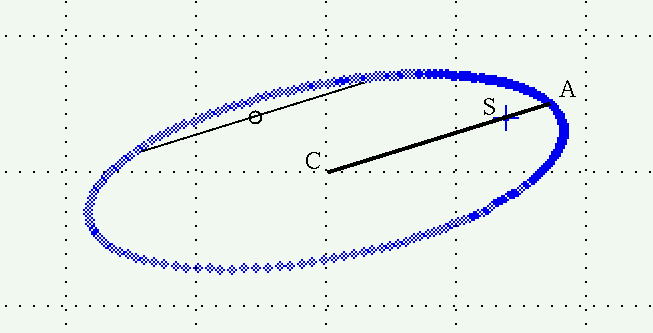
We're ready to build the auxiliary ellipse graphically. It will take a bit of repetitive actions, but each one is pretty simple. We can mark a single point on the auxiliary ellipse by doing this:
- pick any point X on the projected ellipse
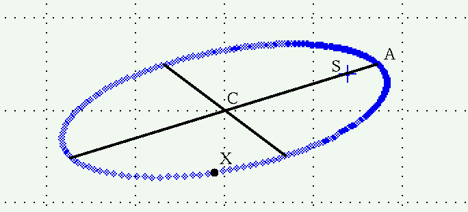
- draw a line parallel to the true minor axis from X to the projection of the true major axis
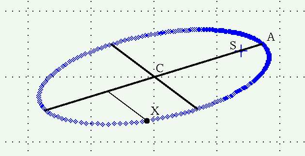
- measure the length of this line; call it \(\mathbf{d}\)
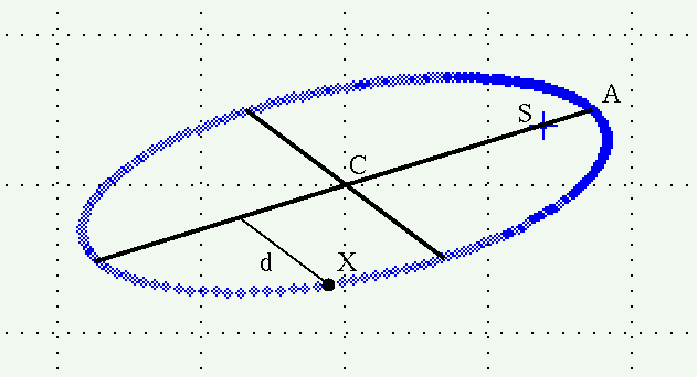
- extend this line outside the ellipse so that its length is \(\mathbf{kd}\), where \(\mathbf{k}\) is the constant you determined back in step 3a
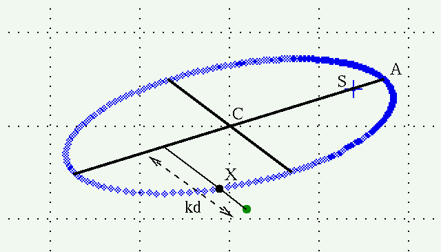
If we repeat this procedure at different locations around the projected ellipse, we can build up a set of points which define the auxiliary ellipse.
We can now connect the dots to draw the auxiliary ellipse.
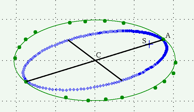
Note that the auxiliary ellipse
- shares the same center as the projected orbit
- touches the projected orbit on the projected major axis
- may have principal axes rotated relative to the projected orbit's principal axes
Step 4: find the true semimajor axis a of the orbit
Once you have drawn the auxiliary ellipse, measure its semimajor (\(\alpha\)) and semiminor (\(\beta\)) axes.

Now, recall that the auxiliary ellipse is a projection of the eccentric circle. The eccentric circle had the same radius as the true orbit's semimajor axis \(\mathbf{a}\). When we tilted it, we squished that circle into an ellipse ... EXCEPT along the axis of rotation. So the longest diameter of the auxiliary ellipse must still be the same as the original radius of the eccentric circle; but that's also the same as the semimajor axis \(\mathbf{a}\) of the true orbit. To make a long story short, the semimajor axis \(\mathbf{a}\) of the auxiliary ellipse is the same as the semimajor axis \(\mathbf{a}\) of the true orbit!
At this point, if all we desire is the total mass of the binary star system, we can quit; after all, we now have the true semimajor axis \(\mathbf{a}\) of the binary star orbit, which we can plug into Kepler's Third Law.
Step 5: find the inclination angle i
Again consider the eccentric circle we drew around the true orbit. When the circle is tilted by the inclination angle \(\mathbf{i}\), it becomes squished into an ellipse. The maximum amount of squishing occurs perpendicular to the axis of rotation, where the original radius \(\mathbf{a}\) shrinks by a factor \(cos(i)\) and turns into the semiminor axis (\(\beta\)) of the auxiliary ellipse. The minimum amount of squishing, as mentioned above, occurs along the axis of rotation: the original radius \(\mathbf{a}\) is unchanged and exactly the same as the semimajor axis (\(\alpha\)) of the auxiliary ellipse.
In other words,
\[\frac{\beta}{\alpha} = \frac{a \cos(i)}{a} = cos(i) \nonumber \]
Aha! We can calculate the inclination angle i from the ratio of the semimajor and semiminor axes of the auxiliary ellipse.
Step 6: find the line of nodes
The last thing we need to know to recover the orientation of the true orbit in space is the axis around which the orbit has been tilted by the inclination angle. Another name for this axis is the line of nodes. How can we describe this? And how can we recover it from the observed orbit?
Go back to the original orbit, observed face-on. Let the the line of nodes be shown as the line connecting the \(\Omega\); it always runs through the position of the primary star, S.
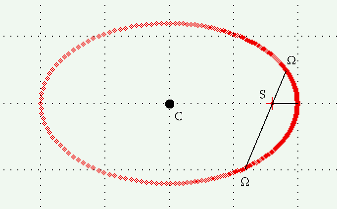
We can define an angle, \(\mathbf{\omega}\) (omega), as the angle between the perihelion vector and the line from the primary star to the nearer node N.
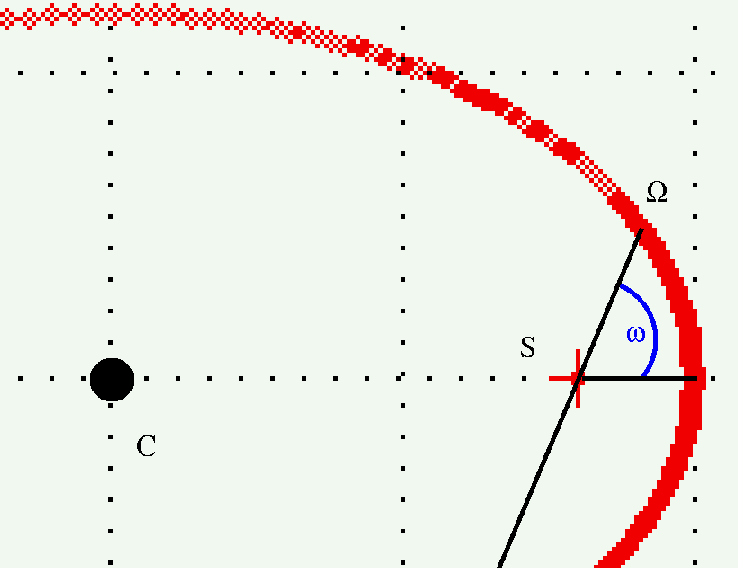
This angle is called the argument of perihelion.
How can we find this angle in the observed orbit? Let's return to our diagram of the observed orbit and auxiliary ellipse.
.gif?revision=1)
As mentioned above, the longest axis of the auxiliary ellipse is the only diameter of the eccentric circle not squished by the tilt of the orbit to our line of sight. Since that tilt was made around the line of nodes, that means that the major axis of the auxiliary ellipse is parallel to the line of nodes.
So, the line which is parallel to the major axis of the auxiliary ellipse, and which passes through the primary star S, must be the line of nodes. Let's draw this line on the projected orbit.
Now zoom in on the portion of the orbit close to perihelion. The line of nodes meets the projected orbit at a location we'll call \(\mathbf{\Omega}\) (capital Omega). In this projected view, we can measure the angle from node \(\mathbf{\Omega}\) to the primary star S and back to the perihelion A; call this angle \(\mathbf{\lambda}\).
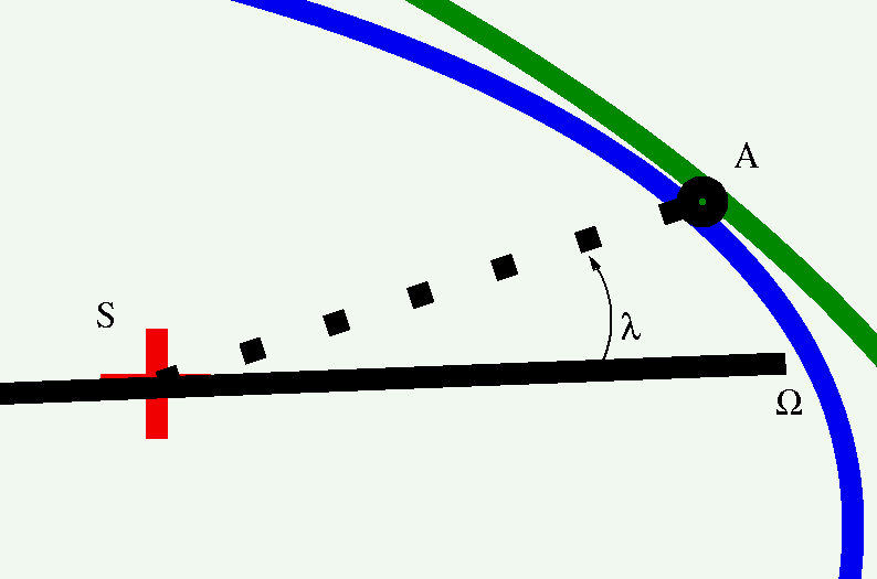
This isn't quite what we want, because we're looking on a projected version of the true orbit. If we correct for the tilt, we can recover the true argument of perihelion:
\[\tan \omega=\frac{\tan \lambda}{\cos i} \nonumber \]
Summary
Phew. That's it. We now know the following properties of the true binary orbit:
- eccentricity \(\mathbf{e}\)
- semimajor axis \(\mathbf{a}\)
- inclination angle \(\mathbf{i}\)
- the line of nodes \(\mathbf{\Omega}\)
- argument of perihelion \(\mathbf{ω}\)
These are five of the seven parameters which completely describe an orbit. The remaining two are the period \(\mathbf{P}\) and the time of perihelion passage \(\mathbf{T}\), which we can determine based on the times associated with all the observations.
Remember, if all we want is the total mass of the two stars, all we need to calculate is \(\mathbf{a}\).
For more information
- The on-line lecture notes of J. B. Tatum contain a chapter on deriving the true properties of an observed orbit.
- The Textbook on Spherical Astronomy by W. M. Smart contains a chapter on the analysis of binary star orbits.
- The RIT Library has a copy of the book The Binary Stars by Robert Grant Aitken. It's a goldmine of information, despite being originally published in 1935.