
35: The Curve of Growth
- Page ID
- 24389

\( \newcommand{\vecs}[1]{\overset { \scriptstyle \rightharpoonup} {\mathbf{#1}} } \)
\( \newcommand{\vecd}[1]{\overset{-\!-\!\rightharpoonup}{\vphantom{a}\smash {#1}}} \)
\( \newcommand{\dsum}{\displaystyle\sum\limits} \)
\( \newcommand{\dint}{\displaystyle\int\limits} \)
\( \newcommand{\dlim}{\displaystyle\lim\limits} \)
\( \newcommand{\id}{\mathrm{id}}\) \( \newcommand{\Span}{\mathrm{span}}\)
( \newcommand{\kernel}{\mathrm{null}\,}\) \( \newcommand{\range}{\mathrm{range}\,}\)
\( \newcommand{\RealPart}{\mathrm{Re}}\) \( \newcommand{\ImaginaryPart}{\mathrm{Im}}\)
\( \newcommand{\Argument}{\mathrm{Arg}}\) \( \newcommand{\norm}[1]{\| #1 \|}\)
\( \newcommand{\inner}[2]{\langle #1, #2 \rangle}\)
\( \newcommand{\Span}{\mathrm{span}}\)
\( \newcommand{\id}{\mathrm{id}}\)
\( \newcommand{\Span}{\mathrm{span}}\)
\( \newcommand{\kernel}{\mathrm{null}\,}\)
\( \newcommand{\range}{\mathrm{range}\,}\)
\( \newcommand{\RealPart}{\mathrm{Re}}\)
\( \newcommand{\ImaginaryPart}{\mathrm{Im}}\)
\( \newcommand{\Argument}{\mathrm{Arg}}\)
\( \newcommand{\norm}[1]{\| #1 \|}\)
\( \newcommand{\inner}[2]{\langle #1, #2 \rangle}\)
\( \newcommand{\Span}{\mathrm{span}}\) \( \newcommand{\AA}{\unicode[.8,0]{x212B}}\)
\( \newcommand{\vectorA}[1]{\vec{#1}} % arrow\)
\( \newcommand{\vectorAt}[1]{\vec{\text{#1}}} % arrow\)
\( \newcommand{\vectorB}[1]{\overset { \scriptstyle \rightharpoonup} {\mathbf{#1}} } \)
\( \newcommand{\vectorC}[1]{\textbf{#1}} \)
\( \newcommand{\vectorD}[1]{\overrightarrow{#1}} \)
\( \newcommand{\vectorDt}[1]{\overrightarrow{\text{#1}}} \)
\( \newcommand{\vectE}[1]{\overset{-\!-\!\rightharpoonup}{\vphantom{a}\smash{\mathbf {#1}}}} \)
\( \newcommand{\vecs}[1]{\overset { \scriptstyle \rightharpoonup} {\mathbf{#1}} } \)
\(\newcommand{\longvect}{\overrightarrow}\)
\( \newcommand{\vecd}[1]{\overset{-\!-\!\rightharpoonup}{\vphantom{a}\smash {#1}}} \)
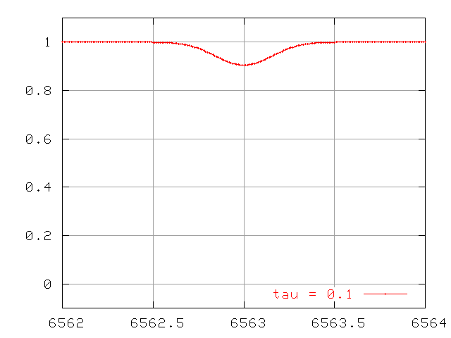
\(\newcommand{\avec}{\mathbf a}\) \(\newcommand{\bvec}{\mathbf b}\) \(\newcommand{\cvec}{\mathbf c}\) \(\newcommand{\dvec}{\mathbf d}\) \(\newcommand{\dtil}{\widetilde{\mathbf d}}\) \(\newcommand{\evec}{\mathbf e}\) \(\newcommand{\fvec}{\mathbf f}\) \(\newcommand{\nvec}{\mathbf n}\) \(\newcommand{\pvec}{\mathbf p}\) \(\newcommand{\qvec}{\mathbf q}\) \(\newcommand{\svec}{\mathbf s}\) \(\newcommand{\tvec}{\mathbf t}\) \(\newcommand{\uvec}{\mathbf u}\) \(\newcommand{\vvec}{\mathbf v}\) \(\newcommand{\wvec}{\mathbf w}\) \(\newcommand{\xvec}{\mathbf x}\) \(\newcommand{\yvec}{\mathbf y}\) \(\newcommand{\zvec}{\mathbf z}\) \(\newcommand{\rvec}{\mathbf r}\) \(\newcommand{\mvec}{\mathbf m}\) \(\newcommand{\zerovec}{\mathbf 0}\) \(\newcommand{\onevec}{\mathbf 1}\) \(\newcommand{\real}{\mathbb R}\) \(\newcommand{\twovec}[2]{\left[\begin{array}{r}#1 \\ #2 \end{array}\right]}\) \(\newcommand{\ctwovec}[2]{\left[\begin{array}{c}#1 \\ #2 \end{array}\right]}\) \(\newcommand{\threevec}[3]{\left[\begin{array}{r}#1 \\ #2 \\ #3 \end{array}\right]}\) \(\newcommand{\cthreevec}[3]{\left[\begin{array}{c}#1 \\ #2 \\ #3 \end{array}\right]}\) \(\newcommand{\fourvec}[4]{\left[\begin{array}{r}#1 \\ #2 \\ #3 \\ #4 \end{array}\right]}\) \(\newcommand{\cfourvec}[4]{\left[\begin{array}{c}#1 \\ #2 \\ #3 \\ #4 \end{array}\right]}\) \(\newcommand{\fivevec}[5]{\left[\begin{array}{r}#1 \\ #2 \\ #3 \\ #4 \\ #5 \\ \end{array}\right]}\) \(\newcommand{\cfivevec}[5]{\left[\begin{array}{c}#1 \\ #2 \\ #3 \\ #4 \\ #5 \\ \end{array}\right]}\) \(\newcommand{\mattwo}[4]{\left[\begin{array}{rr}#1 \amp #2 \\ #3 \amp #4 \\ \end{array}\right]}\) \(\newcommand{\laspan}[1]{\text{Span}\{#1\}}\) \(\newcommand{\bcal}{\cal B}\) \(\newcommand{\ccal}{\cal C}\) \(\newcommand{\scal}{\cal S}\) \(\newcommand{\wcal}{\cal W}\) \(\newcommand{\ecal}{\cal E}\) \(\newcommand{\coords}[2]{\left\{#1\right\}_{#2}}\) \(\newcommand{\gray}[1]{\color{gray}{#1}}\) \(\newcommand{\lgray}[1]{\color{lightgray}{#1}}\) \(\newcommand{\rank}{\operatorname{rank}}\) \(\newcommand{\row}{\text{Row}}\) \(\newcommand{\col}{\text{Col}}\) \(\renewcommand{\row}{\text{Row}}\) \(\newcommand{\nul}{\text{Nul}}\) \(\newcommand{\var}{\text{Var}}\) \(\newcommand{\corr}{\text{corr}}\) \(\newcommand{\len}[1]{\left|#1\right|}\) \(\newcommand{\bbar}{\overline{\bvec}}\) \(\newcommand{\bhat}{\widehat{\bvec}}\) \(\newcommand{\bperp}{\bvec^\perp}\) \(\newcommand{\xhat}{\widehat{\xvec}}\) \(\newcommand{\vhat}{\widehat{\vvec}}\) \(\newcommand{\uhat}{\widehat{\uvec}}\) \(\newcommand{\what}{\widehat{\wvec}}\) \(\newcommand{\Sighat}{\widehat{\Sigma}}\) \(\newcommand{\lt}{<}\) \(\newcommand{\gt}{>}\) \(\newcommand{\amp}{&}\) \(\definecolor{fillinmathshade}{gray}{0.9}\)So, we measure a stellar spectrum, and notice a very weak absorption line. This happens to correspond to an absorption line which has an optical depth \(\mathbf{τ = 0.1}\). That means that most of the photons of the central wavelength (6563 Angstroms in the example below) produced within the photosphere manage to escape before being scattered or absorbed.
Thermally broadened lines
For ordinary stars like the Sun, weak lines are dominated by Doppler broadening. The width of the line is caused by random motions of the atoms absorbing the light. How does Doppler broadening grow as we increase the number of absorbing atoms?
Recall that the optical depth can be defined as
\[\begin{aligned} \frac{I}{I_{0}} &=e^{-\kappa \rho s} \\ &=e^{-\tau} \end{aligned} \nonumber \]
So, if we double the density \(\mathbf{ρ}\) (and hence number of atoms), we double the optical depth. How does this affect the equivalent width? For thermal broadening, one can calculate the change in the absorption profile and find ....
At first, this doubling of the optical depth causes a doubling of the the equivalent width of the line
- There is a linear relationship between number of atoms and equivalent width for an optically thin line.
But as the line becomes optically thick, the equivalent width no longer grows in step with the optical depth (and number of atoms):
And for lines which are VERY optically thick, the equivalent width due to thermal motions grows very slowly ....
The problem here is that the only way the equivalent width can increase is for the wings to grow. The wings of this line are due to atoms which are moving either towards or away from the observer. How many atoms are moving really fast? The distributions of speeds in an ordinary cloud of gas obey a Maxwellian distribution:
\[\text{Prob}(v) = 4 \pi \left( \frac{M}{2\pi R T} \right)^{3/2}v^2e^{-Mv^2/2RT} \nonumber \]
The number of atoms with speed \(\mathbf{v}\) falls off at high speeds as
\[\text{Prob}(v) \propto v^2 e^{-v^2} \nonumber \]
It's easier to read the numbers on a logarithmic plot:
In brief, the number of atoms with very high speeds -- and hence very large Doppler shifts -- decreases very rapidly. There just aren't many atoms available to grow the wings.
Exercise \(\PageIndex{1}\)
There are very, very roughly 10^(38) hydrogen atoms in the entire solar photosphere. Using the graph above, estimate
- the typical speed of a hydrogen atom
- the total number of hydrogen atoms with this speed
- the Doppler shift in an H-alpha line due to this motion
- the total number of hydrogen atoms which would cause a Doppler shift twice as large
- the total number of hydrogen atoms which would cause a Doppler shift four times as large
- the total number of hydrogen atoms which would cause a Doppler shift eight times as large
Remember, these are TOTAL number of atoms in the entire photosphere!
Pressure and collisionally broadened lines
The pressure and collisional (and the natural broadening) processes all produce a Lorentzian line profile: the optical depth \(\mathbf{τ}\) changes with wavelength as
\[\tau(\lambda) = \tau(\lambda_0) \left(\frac{Q^2}{(\lambda - \lambda_0)^2 + Q^2} \right) \nonumber \]
At large distances from the line center, this optical depth goes like
\[\tau \propto (\lambda - \lambda_0)^{-2} \nonumber \]
There is no exponential involved this time, so the function falls off much more slowly than that for thermal broadening. As a result, the lines have much wider wings.
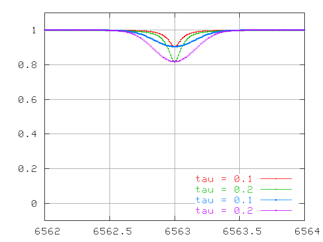
Watch the lines change at small optical depth ...
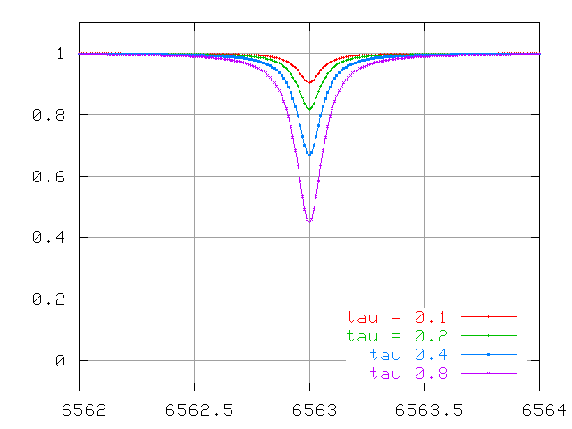
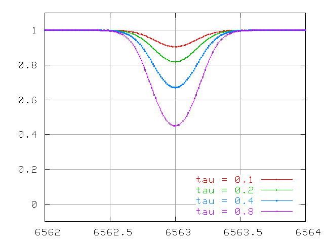
... optical depths of order unity ....
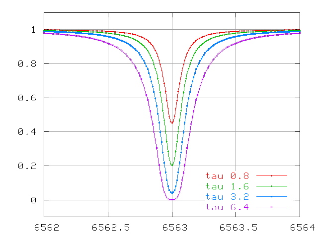
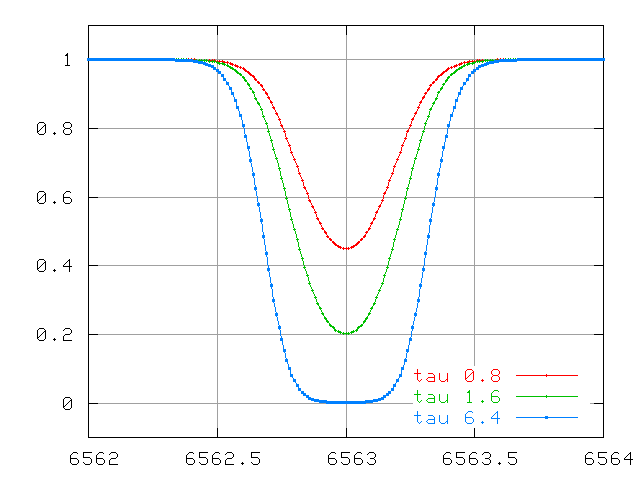
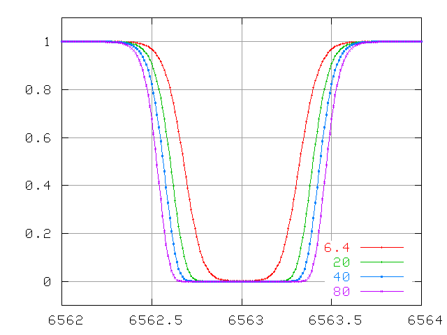
... and very large optical depths.
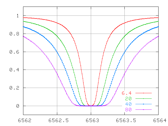
The wings continue to increase in width quickly, even after the line becomes saturated.
Compare the behavior of Doppler-broadened and collisionally-broadened lines at small optical depth
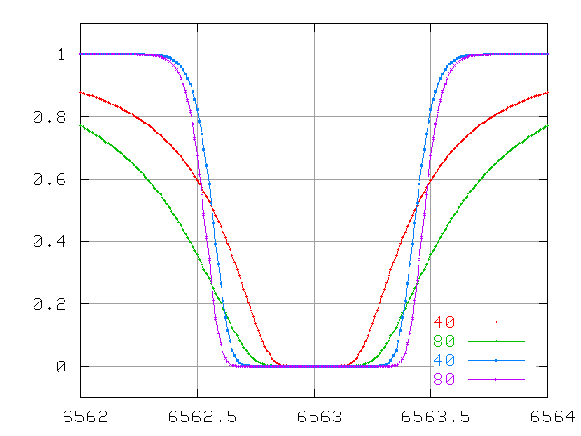
and at large optical depth.
The curve of growth
The combination of both Doppler and collisional processes leads to a complex change in the equivalent width of a spectral line as the optical depth increases. Let's use \(\mathbf{N}\) to denote the number of absorbing atoms, and \(\mathbf{W}\) the equivalent width of the line.
- when there are few absorbers, the optical depth is small;
\[W \propto N \nonumber \]
- after the line saturates (when \(\mathbf{τ > 5}\) or so), the Doppler wings barely change as the number of atoms grow. To a fair approximation,
\[W \propto \sqrt{\ln N} \nonumber \]
- eventually, the wings due to collisional broadening overwhelm the Doppler wings, even though the collisional term is much smaller near the line center. To a decent approximation,
\[W \propto \sqrt{N} \nonumber \]
A plot of the equivalent width \(\mathbf{W}\) as a function of the number of absorbing atoms \(\mathbf{N}\) is called the curve of growth.
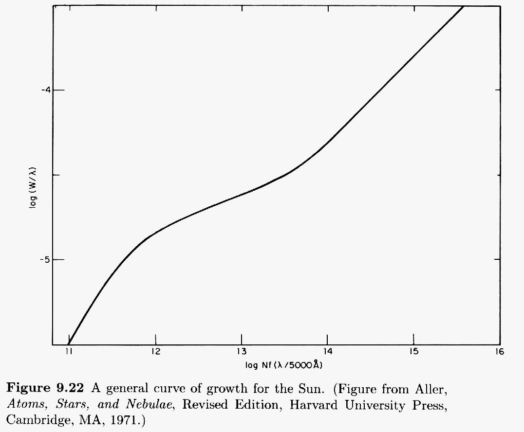
This figure taken from Carroll and Ostlie, "An Introduction to Modern Astrophysics" (Addison-Wesley 1996)
You can see the three different regimes: optically thin, saturated, and REALLY saturated.
Using the curve of growth
If you look closely at the figure above, you'll see that the axes are a bit peculiar.
- The vertical axis is the logarithm of (equivalent width divided by central wavelength). That means we can apply this graph to any line, not just one specific transition.The horizontal axis is the logarithm of (\(\mathbf{N}\) times \(\mathbf{f}\) times (wavelength divided by 5000 Angstroms). Let's take this apart:
- The final piece, (wavelength divided by 5000 Angstroms), again permits us to adjust this graph to fit any absorption line.
- The \(\mathbf{N}\) refers to the column density of atoms which are in the proper state to absorb the photon of interest. For example, if we are studying the hydrogen Balmer alpha line, then \(\mathbf{N}\) is the number of hydrogen atoms in the n=2 state. The "column density" simply counts the number of atoms which appear in an imaginary cylindrical tube of cross-section one square centimeter running from your eye to the photosphere. We are interested in a cross-section, after all, since we are watching light from a background source pass through some column of cooler gas. What matters is not the length of the column of absorbing gas, or the density of the gas within, but the combination of those two factors.
- The \(\mathbf{f}\) refers to the oscillator strength of the atomic transition in question. The larger the value of \(\mathbf{f}\), the more likely the transition will occur. You can look up values of oscillator strengths for any particular transition in many references.
So, how do we use this? The basic idea is
- observe some absorption line. Measure its equivalent width \(\mathbf{W}\)
- locate the position of this line on the curve of growth
- read the horizontal value from the graph
- look up the oscillator strength \(\mathbf{f}\) for the transition in question
- calculate the column density of atoms in the "ready-to-absorb" state
- use the Boltzmann and Saha equations to determine the fraction of all atoms which are in the "ready-to-absorb" state
- compute the total column density of atoms
Let's try it! Below is a section of the spectrum near the 5890 line of neutral sodium, produced when a sodium atom jumps from the ground state 3s1 to the excited state 3p1.
The oscillator strength for this transition is \(\mathbf{f = 0.645}\).
Exercise \(\PageIndex{2}\)
- Measure the equivalent width of this sodium absorption line
- Find its location on the curve of growth
- Calculate the column density of sodium atoms in the ground state
- Estimate the ratio of sodium atoms in the ground state to sodium atoms in excited states
- Estimate the ratio of neutral sodium atoms to ionized sodium atoms; you'll need to know the partition functions for neutral and ionized sodium (2.4 and 1.0, respectively), and the ionization energy for sodium (about 5.1 eV).
- Compute the total column density of sodium atoms in the sun's photosphere. Note: in class, the column density below was misprinted: it was a factor of 1000 too large
- The column density of hydrogen atoms is about \(6.6 \times 10^{23}\); what is the abundance of sodium relative to hydrogen?
- Answer
For more information
- J. B. Tatum's course on "Stellar Atmospheres" is an excellent resource, and it's on line!
- Atomic spectral line list by Hirata and Horaguchi contains a wealth of information (including oscillator strength values) for thousands of lines.