
5.4.3: Plane discs


- Last updated
- Mar 5, 2022
- Save as PDF

( \newcommand{\kernel}{\mathrm{null}\,}\)
FIGURE V.2A
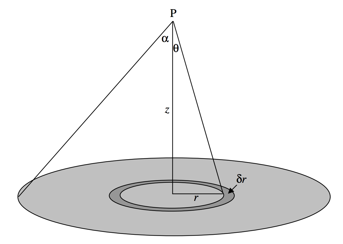
Consider a disc of surface density (mass per unit area) σ, radius a, and a point P on its axis at a distance z from the disc. The contribution to the field from an elemental annulus, radii r, r+δr, mass 2πσ r δr is (from Equation 5.4.1)
δg=2πGσzrδr(z2+r2)3/2.
To find the field from the entire disc, just integrate from r=0 to a, and, if the disc is of uniform surface density, σ will be outside the integral sign. It will be easier to integrate with respect to θ (from 0 to α), where r=ztanθ. You should get
g=2πGσ(1−cosα),
or, with M=πa2σ,
g=2GM(1−cosα)a2.
Now 2π(1−cosα) is the solid angle ω subtended by the disc at P. (Convince yourself of this – don’t just take my word for it.) Therefore
g=Gσω.
This expression is also the same for a uniform plane lamina of any shape, for the downward component of the gravitational field. For, consider figure V.3.
The downward component of the field due to the element δA is GσδAcosθr2=Gσδω. Thus, if you integrate over the whole lamina, you arrive at Gσω.
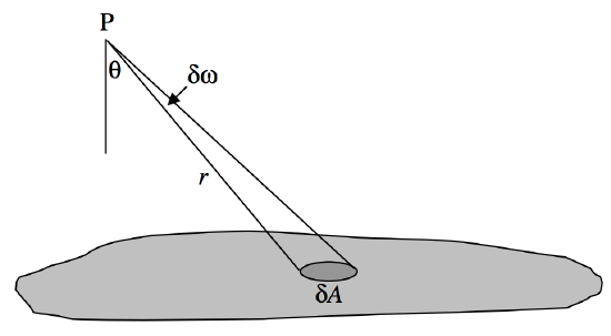
FIGURE 5.3
Returning to Equation 5.4.8, we can write the Equation in terms of z rather than α. If we express g in units of GM/a2 and z in units of a, the Equation becomes
g=2(1−z√1+z2).
This is illustrated in figure V.4.
FIGURE V.4
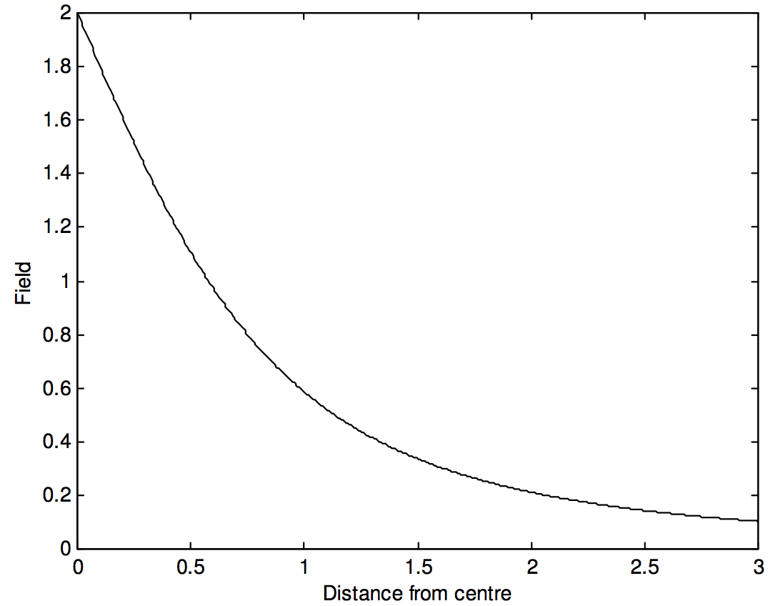
The field is greatest immediately above the disc. On the opposite side of the disc, the field changes direction. In the plane of the disc, at the centre of the disc, the field is zero. For more on this, see Subsection 5.4.7.
If you are calculating the field on the axis of a disc that is not of uniform surface density, but whose surface density varies as σ(r), you will have to calculate
M=2π∫a0σ(r)rdr
and g=2πGz∫a0σ(r)rdr(z2+r2)3/2.
You could try, for example, some of the following forms for σ(r):
σ0(1−kra),σ0(1−kr2a),σ0√1−kra,σ0√1−kr2a2.
If you are interested in galaxies, you might want to try modelling a galaxy as a central spherical bulge of density ρ and radius a1, plus a disc of surface density σ(r) and radius a2, and from there you can work your way up to more sophisticated models.
In this section we have calculated the field on the axis of a disc. As soon as you move off axis, it becomes much more difficult.
Exercise. Starting from Equations 5.4.1 and 5.4.10, show that at vary large distances along the axis, the fields for a ring and for a disc each become GM/z2. All you have to do is to expand the expressions binomially in a/z. The field at a large distance r from any finite object will approach GM/r2.