10.9: Worked Examples

Problem Solving Strategies

When solving problems involving changing momentum in a system, we shall employ our general problem solving strategy involving four basic steps:

1. Understand – get a conceptual grasp of the problem.

2. Devise a Plan - set up a procedure to obtain the desired solution.

3. Carry our your plan – solve the problem!

4. Look Back – check your solution and method of solution.

We shall develop a set of guiding ideas for the first two steps.

1. Understand – get a conceptual grasp of the problem

The first question you should ask is whether or not momentum is constant in some system that is changing its state after undergoing an interaction. First you must identify the objects that compose the system and how they are changing their state due to the interaction. As a guide, try to determine which objects change their momentum in the course of interaction. You must keep track of the momentum of these objects before and after any interaction. Second, momentum is a vector quantity so the question of whether momentum is constant or not must be answered in each relevant direction. In order to determine this, there are two important considerations. You should identify any external forces acting on the system. Remember that a non-zero external force will cause the momentum of the system to change, (Equation (10.4.9) above),

\[\overrightarrow{\mathbf{F}}^{e x t}=\frac{d \overrightarrow{\mathbf{p}}_{\mathrm{sys}}}{d t} \nonumber \]

Equation (10.9.1) is a vector equation; if the external force in some direction is zero, then the change of momentum in that direction is zero. In some cases, external forces may act but the time interval during which the interaction takes place is so small that the impulse is small in magnitude compared to the momentum and might be negligible. Recall that the average external impulse changes the momentum of the system

\[\overrightarrow{\mathbf{I}}=\overrightarrow{\mathbf{F}}^{\mathrm{ext}} \Delta t_{\mathrm{int}}=\Delta \overrightarrow{\mathbf{p}}_{\mathrm{sys}} \nonumber \]

If the interaction time is small enough, the momentum of the system is constant, \(\Delta \overrightarrow{\mathbf{p}} \rightarrow \overrightarrow{\mathbf{0}}\) If the momentum is not constant then you must apply either Equation (10.9.1) or Equation (10.9.2). If the momentum of the system is constant, then you can apply Equation (10.7.5),

\[\overrightarrow{\mathbf{p}}_{\mathrm{sys}, i}=\overrightarrow{\mathbf{p}}_{\mathrm{sys}, f} \nonumber \]

If there is no net external force in some direction, for example the x -direction, the component of momentum is constant in that direction, and you must apply

\[\mathbf{p}_{\mathrm{sys}, x, i}=\mathbf{p}_{\mathrm{sys},x, f} \nonumber \]

2. Devise a Plan - set up a procedure to obtain the desired solution

Draw diagrams of all the elements of your system for the two states immediately before and after the system changes its state. Choose symbols to identify each mass and velocity in the system. Identify a set of positive directions and unit vectors for each state. Choose your symbols to correspond to the state and motion (this facilitates an easy interpretation, for example \(\left(v_{x, i}\right)_{1}\) represents the x -component of the velocity of object 1 in the initial state and \(\left(v_{x, f}\right)_{1}\) represents the x -component of the velocity of object 1 in the final state). Decide whether you are using components or magnitudes for your velocity symbols. Since momentum is a vector quantity, identify the initial and final vector components of the momentum. We shall refer to these diagrams as momentum flow diagrams. Based on your model you can now write expressions for the initial and final momentum of your system. As an example in which two objects are moving only in the x -direction, the initial x -component of the momentum is

\[p_{\text {sys }, x, i}=m_{1}\left(v_{x, i}\right)_{1}+m_{2}\left(v_{x, i}\right)_{2}+\cdots \nonumber \]

The final x -component of the momentum is

\[p_{\text {sys, } x, f}=m_{1}\left(v_{x, f}\right)_{1}+m_{2}\left(v_{x, f}\right)_{2}+\cdots \nonumber \]

If the x -component of the momentum is constant then

\[\mathbf{p}_{\mathrm{sys}, x, i}=\mathbf{p}_{\mathrm{sys},x, f} \nonumber \]

We can now substitute Equations (10.9.5) and (10.9.6) into Equation (10.9.7), yielding

\[m_{1}\left(v_{x, i}\right)_{1}+m_{2}\left(v_{x, i}\right)_{2}+\cdots=m_{1}\left(v_{x, f}\right)_{1}+m_{2}\left(v_{x, f}\right)_{2}+\cdots \nonumber \]

Equation (10.9.8) can now be used for any further analysis required by a particular problem. For example, you may have enough information to calculate the final velocities of the objects after the interaction. If so then carry out your plan and check your solution, especially dimensions or units and any relevant vector directions.

Example 10.5 Exploding Projectile

An instrument-carrying projectile of mass \(m_{1}\) accidentally explodes at the top of its trajectory. The horizontal distance between launch point and the explosion is \(x_{i}\). The projectile breaks into two pieces that fly apart horizontally. The larger piece, \(m_{3}\) has three times the mass of the smaller piece, \(m_{2}\). To the surprise of the scientist in charge, the smaller piece returns to earth at the launching station. Neglect air resistance and effects due to the earth’s curvature. How far away, \(x_{3, f}\), from the original launching point does the larger piece land?

Figure 10.8 Exploding projectile trajectories

Solution: We can solve this problem two different ways. The easiest approach is utilizes the fact that the external force is the gravitational force and therefore the center of mass of the system follows a parabolic trajectory. From the information given in the problem \(m_{2}=m_{1} / 4\) and \(m_{3}=3 m_{1} / 4\). Thus when the two objects return to the ground the center of mass of the system has traveled a distance \(R_{c m}=2 x_{i}\). We now use the definition of center of mass to find where the object with the greater mass hits the ground. Choose an origin at the starting point. The center of mass of the system is given by

\[\overrightarrow{\mathbf{R}}_{c m}=\frac{m_{2} \overrightarrow{\mathbf{r}}_{2}+m_{3} \overrightarrow{\mathbf{r}}_{3}}{m_{2}+m_{3}} \nonumber \]

So when the objects hit the ground \(\overrightarrow{\mathbf{R}}_{c m}=2 x_{i} \hat{\mathbf{i}}\), the object with the smaller mass returns to the origin, \(\overrightarrow{\mathbf{r}}_{2}=\overrightarrow{\mathbf{0}}\), and the position vector of the other object is \(\overrightarrow{\mathbf{r}}_{3}=x_{3, f} \hat{\mathbf{i}}\). So using the definition of the center of mass,

\[2 x_{i} \hat{\mathbf{i}}=\frac{\left(3 m_{1} / 4\right) x_{3, f} \hat{\mathbf{i}}}{m_{1} / 4+3 m_{1} / 4}=\frac{\left(3 m_{1} / 4\right) x_{3, f} \hat{\mathbf{i}}}{m_{1}}=\frac{3}{4} x_{3, f} \hat{\mathbf{i}} \nonumber \]

Therefore

\[x_{3, f}=\frac{8}{3} x_{i} \nonumber \]

Note that the neither the vertical height above ground nor the gravitational acceleration g entered into our solution.

Alternatively, we can use conservation of momentum and kinematics to find the distance traveled. Because the smaller piece returns to the starting point after the collision, the velocity of the smaller piece immediately after the explosion is equal to the negative of the velocity of original object immediately before the explosion. Because the collision is instantaneous, the horizontal component of the momentum is constant during the collision. We can use this to determine the speed of the larger piece after the collision. The larger piece takes the same amount of time to return to the ground as the projectile originally takes to reach the top of the flight. We can therefore determine how far the larger piece traveled horizontally.

We begin by identifying various states in the problem.

Initial state, time \(t_{0}=0\): the projectile is launched.

State 1 time \(t_{1}\): the projectile is at the top of its flight trajectory immediately before the explosion. The mass is \(m_{1}\) and the velocity of the projectile is \(\overrightarrow{\mathbf{v}}_{1}=v_{1} \hat{\mathbf{i}}\).

State 2 time \(t_{2}\): immediately after the explosion, the projectile has broken into two pieces, one of mass \(m_{2}\) moving backwards (in the negative x -direction) with velocity \(\overrightarrow{\mathbf{v}}_{2}=-\overrightarrow{\mathbf{v}}_{1}\). The other piece of mass \(m_{3}\) is moving in the positive x -direction with velocity \(\overrightarrow{\mathbf{v}}_{3}=v_{3} \hat{\mathbf{i}}\), (Figure 10.8).

State 3: the two pieces strike the ground at time \(t_{f}=2 t_{1}\) one at the original launch site 1 and the other at a distance, \(x_{3, f}\) from the launch site, as indicated in Figure 10.8. The pieces take the same amount of time to reach the ground \(\Delta t=t_{1}\) because both pieces are falling from the same height as the original piece reached at time \(t_{1}\) and each has no component of velocity in the vertical direction immediately after the explosion. The momentum flow diagram with state 1 as the initial state and state 2 as the final state are shown in the upper two diagrams in Figure 10.8.

The initial momentum at time \(t_{1}\) immediately before the explosion is

\[\overrightarrow{\mathbf{p}}^{s s}\left(t_{1}\right)=m_{1} \overrightarrow{\mathbf{v}}_{1} \nonumber \]

The momentum at time \(t_{2}\) immediately after the explosion is

\[\overrightarrow{\mathbf{p}}^{g s}\left(t_{2}\right)=m_{2} \overrightarrow{\mathbf{v}}_{2}+m_{3} \overrightarrow{\mathbf{v}}_{3}=-\frac{1}{4} m_{1} \overrightarrow{\mathbf{v}}_{1}+\frac{3}{4} m_{1} \overrightarrow{\mathbf{v}}_{3} \nonumber \]

During the duration of the instantaneous explosion, impulse due to the external gravitational force may be neglected and therefore the momentum of the system is constant. In the horizontal direction, we have that

\[m_{1} \overrightarrow{\mathbf{v}}_{1}=-\frac{1}{4} m_{1} \overrightarrow{\mathbf{v}}_{1}+\frac{3}{4} m_{1} \overrightarrow{\mathbf{v}}_{3} \nonumber \]

Equation (10.9.11) can now be solved for the velocity of the larger piece immediately after the collision,

\[\overrightarrow{\mathbf{v}}_{3}=\frac{5}{3} \overrightarrow{\mathbf{v}}_{1} \nonumber \]

The larger piece travels a distance

\[x_{3, f}=v_{3} t_{1}=\frac{5}{3} v_{1} t_{1}=\frac{5}{3} x_{i} \nonumber \]

Therefore the total distance the larger piece traveled from the launching station is

\[x_{f}=x_{i}+\frac{5}{3} x_{i}=\frac{8}{3} x_{i} \nonumber \]

in agreement with our previous approach.

Example 10.6 Landing Plane and Sandbag

Figure 10.9 Plane and sandbag

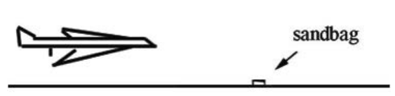
A light plane of mass 1000 kg makes an emergency landing on a short runway. With its engine off, it lands on the runway at a speed of \(40 \mathrm{m} \cdot \mathrm{s}^{-1}\) A hook on the plane snags a cable attached to a 120 kg sandbag and drags the sandbag along. If the coefficient of friction between the sandbag and the runway is \(\mu_{k}=0.4\), and if the plane’s brakes give an additional retarding force of magnitude 1400 N , how far does the plane go before it comes to a stop?

Solution: We shall assume that when the plane snags the sandbag, the collision is instantaneous so the momentum in the horizontal direction remains constant,

\[p_{x, i}=p_{x, 1} \nonumber \]

We then know the speed of the plane and the sandbag immediately after the collision. After the collision, there are two external forces acting on the system of the plane and sandbag, the friction between the sandbag and the ground and the braking force of the runway on the plane. So we can use the Newton’s Second Law to determine the acceleration and then one-dimensional kinematics to find the distance the plane traveled since we can determine the change in kinetic energy.

The momentum of the plane immediately before the collision is

\[\overrightarrow{\mathbf{p}}_{i}=m_{p} v_{p, i} \hat{\mathbf{i}} \nonumber \]

The momentum of the plane and sandbag immediately after the collision is

\[\overrightarrow{\mathbf{p}}_{1}=\left(m_{p}+m_{s}\right) v_{p, 1} \hat{\mathbf{i}} \nonumber \]

Because the x - component of the momentum is constant, we can substitute Equations (10.9.16) and (10.9.17) into Equation (10.9.15) yielding

\[m_{p} v_{p, i}=\left(m_{p}+m_{s}\right) v_{p, 1} \nonumber \]

The speed of the plane and sandbag immediately after the collision is

\[v_{p, 1}=\frac{m_{p} v_{p, i}}{m_{p}+m_{s}} \nonumber \]

The forces acting on the system consisting of the plane and the sandbag are the normal force on the sandbag,

\[\overrightarrow{\mathbf{N}}_{g, s}=N_{g, s} \hat{\mathbf{j}} \nonumber \]

the frictional force between the sandbag and the ground

\[\overrightarrow{\mathbf{f}}_{k}=-f_{k} \hat{\mathbf{i}}=-\mu_{k} N_{g, s} \hat{\mathbf{i}}, \nonumber \]

the braking force on the plane

\[\overrightarrow{\mathbf{F}}_{g, p}=-F_{g, p} \hat{\mathbf{i}} \nonumber \]

and the gravitational force on the system,

\[\left(m_{p}+m_{s}\right) \overrightarrow{\mathbf{g}}=-\left(m_{p}+m_{s}\right) g \hat{\mathbf{j}} \nonumber \]

Newton’s Second Law in the \(\hat{\mathbf{i}}\)-direction becomes

\[-F_{g, p}-f_{k}=\left(m_{p}+m_{s}\right) a_{x} \nonumber \]

If we just look at the vertical forces on the sandbag alone then Newton’s Second Law in the \(\hat{\mathbf{j}}\)-direction becomes

\[N-m_{s} g=0 \nonumber \]

The frictional force on the sandbag is then

\[\overrightarrow{\mathbf{f}}_{k}=-\mu_{k} N_{g, s} \hat{\mathbf{i}}=-\mu_{k} m_{s} g \hat{\mathbf{i}} \nonumber \]

Newton’s Second Law in the \(\hat{\mathbf{1}}\)-direction becomes

\[-F_{g, p}-\mu_{k} m_{s} g=\left(m_{p}+m_{s}\right) a_{x} \nonumber \]

The x -component of the acceleration of the plane and the sand bag is then

\[a_{x}=\frac{-F_{g, p}-\mu_{k} m_{s} g}{m_{p}+m_{s}} \nonumber \]

We choose our origin at the location of the plane immediately after the collision, \(x_{p}(0)=0\). Set t = 0 immediately after the collision. The x -component of the velocity of the plane immediately after the collision is \(v_{x, 0}=v_{p, 1}\). Set \(t=t_{f}\) when the plane just comes to a stop. Because the acceleration is constant, the kinematic equations for the change in velocity is

\[v_{x, f}\left(t_{f}\right)-v_{p, 1}=a_{x} t_{f} \nonumber \]

We can solve this equation for \(t=t_{f}\), where \(v_{x, f}\left(t_{f}\right)=0\)

\[t_{f}=-v_{p, 1} / a_{x} t \nonumber \]

Then the position of the plane when it first comes to rest is

\[x_{p}\left(t_{f}\right)-x_{p}(0)=v_{p, 1} t_{f}+\frac{1}{2} a_{x} t_{f}^{2}=-\frac{1}{2} \frac{v_{p, 1}^{2}}{a_{x}} \nonumber \]

Then using \(x_{p}(0)=0\) and substituting Equation (10.9.26) into Equation (10.9.27) yields

\[x_{p}\left(t_{f}\right)=\frac{1}{2} \frac{\left(m_{p}+m_{s}\right) v_{p, 1}^{2}}{\left(F_{g, p}+\mu_{k} m_{s} g\right)} \nonumber \]

We now use the condition from conservation of the momentum law during the collision, Equation (10.9.19) in Equation (10.9.28) yielding

\[x_{p}\left(t_{f}\right)=\frac{m_{p}^{2} v_{p, i}^{2}}{2\left(m_{p}+m_{s}\right)\left(F_{g, p}+\mu_{k} m_{s} g\right)} \nonumber \]

Substituting the given values into Equation (10.9.28) yields

\[x_{p}\left(t_{f}\right)=\frac{(1000 \mathrm{kg})^{2}\left(40 \mathrm{m} \cdot \mathrm{s}^{-1}\right)^{2}}{2(1000 \mathrm{kg}+120 \mathrm{kg})\left(1400 \mathrm{N}+(0.4)(120 \mathrm{kg})\left(9.8 \mathrm{m} \cdot \mathrm{s}^{-2}\right)\right)}=3.8 \times 10^{2} \mathrm{m} \nonumber \]