13.5: Work done by Non-Constant Forces

Consider a body moving in the x -direction under the influence of a non-constant force in the x -direction, \(\overrightarrow{\mathbf{F}}=F_{x} \hat{\mathbf{i}}\). The body moves from an initial position \(x_{i}\) to a final position \(x_{f}\). In order to calculate the work done by a non-constant force, we will divide up the displacement of the point of application of the force into a large number N of small displacements \(\Delta x_{j}\) where the index j marks the \(j_{th}\) displacement and takes integer values from 1 to N . Let \(\left(F_{x, j}\right)_{\text {ave }}\) denote the average value of the x -component of the force in the displacement interval \(\left[x_{j-1}, x_{j}\right]\). For the \(j_{th}\) displacement interval we calculate the contribution to the work.

\[W_{j}=\left(F_{x, j}\right)_{\text {ave }} \Delta x_{j} \nonumber \]

This contribution is a scalar so we add up these scalar quantities to get the total work

\[W_{N}=\sum_{j=1}^{j=N} W_{j}=\sum_{j=1}^{j=N}\left(F_{x, j}\right)_{\text {ave }} \Delta x_{j} \nonumber \]

The sum in Equation (13.5.2) depends on the number of divisions N and the width of the intervals \(\Delta x_{j}\). In order to define a quantity that is independent of the divisions, we take the limit as \(N \rightarrow \infty\) and \(\left|\Delta x_{j}\right| \rightarrow 0\) for all j . The work is then

\[W=\lim _{N \rightarrow \infty \atop\left|\Delta x_{j}\right| \rightarrow 0} \sum_{j=1}^{j=N}\left(F_{x, j}\right)_{\text {ave }} \Delta x_{j}=\int_{x=x_{i}}^{x=x_{f}} F_{x}(x) d x \nonumber \]

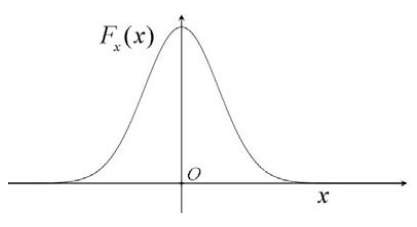
This last expression is the definite integral of the x -component of the force with respect to the parameter x . In Figure 13.5 we graph the x -component of the force as a function of the parameter x . The work integral is the area under this curve between \(x=x_{i}\) and \(x=x_{f}\).

Figure 13.5 Plot of x -component of a sample force \(F_{x}(x)\) as a function of x .

Example \(\PageIndex{1}\): Work done by the Spring Force

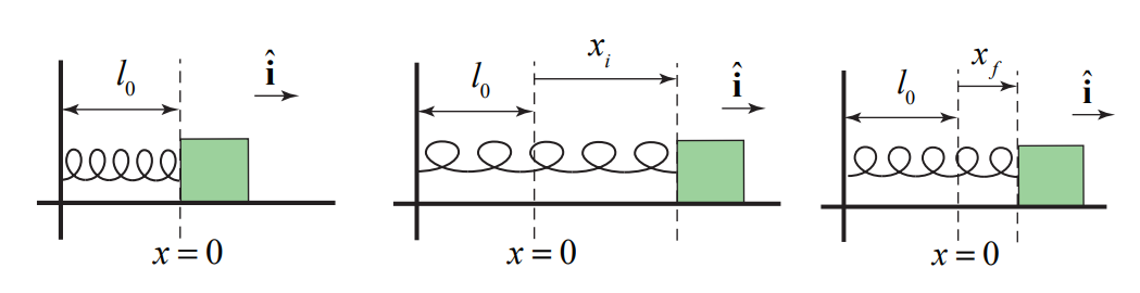
Connect one end of an unstretched spring of length \(l_{0}\) with spring constant k to an object resting on a smooth frictionless table and fix the other end of the spring to a wall. Choose an origin as shown in the figure. Stretch the spring by an amount \(x_{i}\) and release the object. How much work does the spring do on the object when the spring is stretched by an amount \(x_{f}\)?

Figure 13.6 Equilibrium, initial and final states for a spring

Solution

We first begin by choosing a coordinate system with our origin located at the position of the object when the spring is unstretched (or uncompressed). We choose the \(\hat{\mathbf{i}}\) unit vector to point in the direction the object moves when the spring is being stretched. We choose the coordinate function x to denote the position of the object with respect to the origin. We show the coordinate function and free-body force diagram in the figure below.

Figure 13.6a Spring force

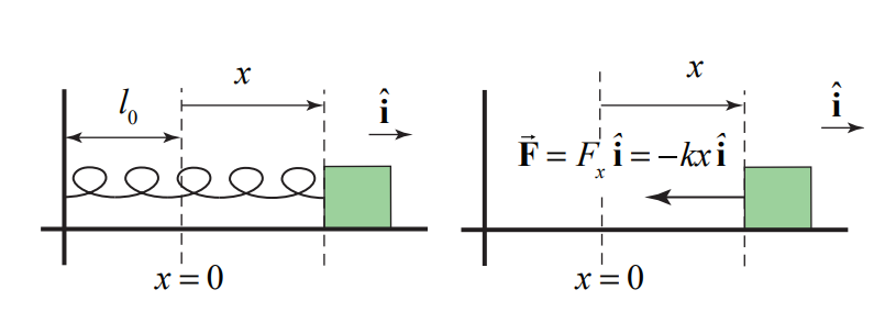
The spring force on the object is given by (Figure 13.6a)

\[\overrightarrow{\mathbf{F}}=F_{x} \hat{\mathbf{i}}=-k x \hat{\mathbf{i}} \nonumber \]

In Figure 13.7 we show the graph of the x -component of the spring force, \(F_{x}(x)\), as a function of x

Figure 13.7 Plot of spring force \(F_{x}(x)\) vs. displacement x

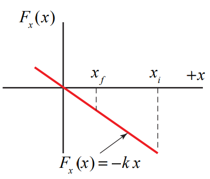
The work done is just the area under the curve for the interval \(x_{i}\) to \(x_{f}\),

\[W=\int_{x^{\prime}=x_{i}}^{x^{\prime}=x_{f}} F_{x}\left(x^{\prime}\right) d x^{\prime}=\int_{x^{\prime}=x_{i}}^{x^{\prime}=x_{f}}-k x^{\prime} d x^{\prime}=-\frac{1}{2} k\left(x_{f}^{2}-x_{i}^{2}\right) \nonumber \]

This result is independent of the sign of \(x_{i}\) and \(x_{f}\) because both quantities appear as squares. If the spring is less stretched or compressed in the final state than in the initial state, then the absolute value, \(\left|x_{f}\right|<\left|x_{i}\right|\) and the work done by the spring force is positive. The spring force does positive work on the body when the spring goes from a state of “greater tension” to a state of “lesser tension.”