5.5: Oblique (Glancing) Elastic Collisions, Alternative Treatment


- Last updated
- Aug 8, 2022
- Save as PDF

( \newcommand{\kernel}{\mathrm{null}\,}\)
In Figure V.3, unlike Figure V.2, the horizontal line is not intended to represent the line of centers. Rather, it is the direction of the initial velocity of m1, and m2 is initially at rest. The second mass m2 is slightly off the line of the velocity of m1. I am assuming that the collision is elastic, so that e=1. In the "before" part of the Figure, I have indicated, as well as the two masses, the position and velocity V of the center of mass C. The velocity of C remains constant, because there are no external forces on the system. I have not drawn C in the "after" part of the Figure, because it would get a little in the way. Think about where it is.
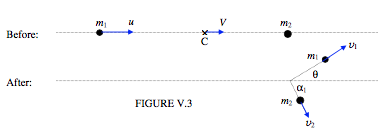
Figure V.3 shows the situation in "laboratory space". (Later, we'll look at the situation referred to a reference frame in which C is at rest – "center of mass space".) The angle θ is the angle through which m1 has been scattered (the "scattering angle"). I have indicated in the Figure how it is related to the α1 and β1 of Section 5.3. Note that m2 (initially stationary) scoots off along the line of centers.
The following two equations express the constancy of linear momentum of the system.
(m1+m2)V=m1u=m1v1cosθ+m2v2cosα1.
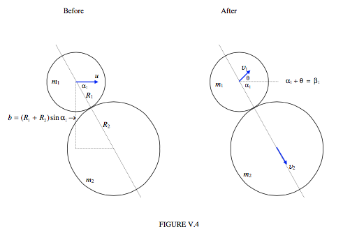
I'm going to draw, in Figure V.4, the situation "close-up", so that you can see the geometry more clearly. Note that the distance b is called the impact parameter. It is the distance by which the two centers would have missed each other had the first particle not been scattered.
In Figure V.5, I draw the situation in center of mass space, in which the center of mass C is stationary. In this reference frame, I just have to subtract V from all the velocities. Note that in center of mass space the speeds of the particles are unaltered by the collision. In center of mass space, m1 is scattered through an angle θ′, and I am going to find a relation between θ′, θ and the mass ratio m2m1.
I shall start with the profound statement that
tanθ=v1sinθv1cosθ
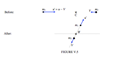
Now v1sinθ is the y-component of the final velocity of m1 in laboratory space. The y-component of the final velocity of m1 in center of mass space is u′sinθ′, and these two are equal, since the y-component of the motion is unaffected by the change of reference frame. Therefore
tanθ=u′sinθ′v1cosθ.
Therefore
v1sinθ=u′sinθ′.
The x-components of the "before" and "after" velocities of m1 are related by
v1cosθ=u′sinθ′+V.
Substitute Equations 5.5.4 and 5.5.6 into Equation 5.5.2 to obtain
tanθ=sinθ′cosθ′+V/u′
But
(m1+m2)V=m1u=m1(u′+V),
from which
Vu′=m1m2.
On substituting this into Equation 5.5.7, we obtain the relation we sought:
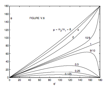
tanθ=sinθ′cosθ′+m1/m2.
This relation is illustrated in Figure V.6 for several mass ratios.
Let us try to interpret the Figure. For m2>m1, any scattering angle, forward or backward, is possible, but for m2<m1, backward scattering is not possible, and forward scattering is possible only up to a maximum. This is only to be expected. Thus for an impact parameter of zero or of R1+R2, and m2<m1, the scattering angle θ must be zero, and therefore for intermediate impact parameters it must go through a maximum. This would be clearer if we could plot the scattering angle versus the impact parameter, and indeed that is something that we shall try to do. In the meantime it is easy to show, by differentiation of Equation 5.5.10 (do it!), that the maximum scattering angle is sin−1μ, where
μ=m2m1.
That is, if the scattered particle is very massive compared with the scattering particle, the maximum scattering angle is small – just to be expected.
I want to do two things now - one, to calculate the scattering angle θ as a function of impact parameter, and two, to calculate v1u as a function of scattering angle. I’m going to start with Equations 5.4.1, 5.4.2 and 5.4.4, except for the following. I’ll assume e=1 (elastic collision), and u2=0(m2 is initially stationary), and β2=0 (since m2 is initially stationary, it must move along the line of centers after collision). Since I want to try to calculate the scattering angle, I’ll write θ+α1 for β1 (see Figure V.4). I’m also going to write r1, r2 and μ for the dimensionless ratios v1u, v2u and m2m1 respectively. With those small changes, Equations 5.4.1, 5.4.2 and 5.4.4 become
r1cos(θ+α1)+μr2=cosα1,
r1sin(θ+α1)=sinα1,
r2−r1cos(θ+α1)=cosα1.
Eliminate r2 from Equations 5.5.11 and 5.5.13 to obtain
r1cos(θ+α1)=Mcosα1,
where
M=1−μ1+μ=m1−m2m1+m2.
If we now eliminate α1 from Equations 5.5.12 and 5.5.14, we obtain the relation between v1u and the scattering angle, which was the second of our two aims above. The elimination is easily done as follows. Expand \sin and cos of θ+α1 in the two equations, divide both sides of each equation by cosα1 and eliminate tanα1 between the two equations. The result is
r21(1+M)cosθ+M=0.
We’ll have a look at this equation in a moment, but in the meantime, instead of eliminating α1 from Equations 5.5.12 and 5.5.14, let’s eliminate r1. This will give us a relation between the scattering angle θ and α1, and, since α1 is closely relation to the impact parameter (see Figure V.4) this will achieve the first of our aims, namely to find the scattering angle as a function of the impact parameter. If you do the algebra, you should find that the relation between θ and α1 is
t=a(1−M)a2+M,
where
t=tanθanda=tanα1.
Now let
b′=bR1+R2
and from Figure V.5 we see that
b′=sinα1.
On elimination of α1 from Equations 5.5.17 and 5.5.19, we obtain the required relation between scattering angle θ and (dimensionless) impact parameter b′:
tanθ=sμb′√1−bt21−μ+2μbt2.
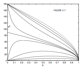
This relation is shown in Figure V .7. The values of the mass ratio μ ( =fracm2m1 ) are (from the
lowest up) 18,14,12,910,1,109,2,4,8 and (dashed) ∞. This Figure is perhaps slightly easier to interpret than Figure V.6. One can see that for μ>1, any scattering angle is possible, but for μ<1, the scattering angle has a maximum possible value, less than 90 °, and the scattering angle is zero for b′ = 0 or 1.
We saw, by differentiation of Equation 5.5.10, that the maximum scattering angle was sin−1μ. Now show the same thing by differentiation of Equation 5.5.20. (This is not so easy, is it?)
Show that the scattering angle is greatest for an impact parameter of
b′=√1−μ2.
Solution
You will notice that, for /( b' = 0/) (head-on collision) the scattering angle changes abruptly from 0 to 180° as the mass ratio changes from less than 1 to more than 1. No problem there. But if the mass ratio is exactly 1 (not the tiniest bit less or the tiniest bit more) the scattering angle is apparently 90°. This may cause some puzzlement until it is realized that for a head-on collision with μ=1 the first sphere comes to a dead halt.
The case of mu=∞ (second sphere immovable) is of some interest. It is easy in that case to calculate how the scattering angle varies with impact parameter for an elastic collision, merely by requiring the scattered sphere to obey the law of reflection, and without any reference to Equation 5.5.20.
Easy Exercise.
Without any reference to Equation 5.5.20, show that, if the second ball is immovable, the scattering angle is related to the impact parameter by
θ=180°−2sin−1b′.
Not-so-easy exercise. Show that, in the limit as μ→∞, Equation 5.5.20 approaches Equation 5.5.22.
In any case, the limiting case as the second sphere becomes immovable is shown as a dashed curve in Figure V.7.
Exercise of Intermediate Difficulty. The mass ratio m2m1 is 0.9, and the scattering angle is 50∘. What was the impact parameter?
Answers
b' = 0.07270 or 0.58540.
We have now dealt with the direction of motion of m1 after scattering as a function of impact parameter. We should now look at the speed of m1 after collision, and this takes us back to Equation 5.5.16, which gives is the speed (r1=v1u) as a function of scattering angle θ. It is 11 quadratic in r1, so, for a given scattering angle there are two possible speeds – which is not surprising, because a given scattering angle can arise from two different impact parameters, as we have just found out. We can conveniently show the relation between r1 and θ simply by plotting the equation in polar coordinates. I’ll re-write the equation here for easy reference:
r21=r1(1+M)cosθ+M=0.
Here, M=1−μ1+μ=11+μ, but I want to write the equation in terms of the mass fractions
q1=m1m1+m2=11+μandq2=m2m1+m2=μ1+μ.
If you work at this for a short while, you will find that Equation 5.5.16 becomes
r21+q21−2r1q1cosθ=q22.
and one is then overcome with an overwhelming desire to draw a triangle:
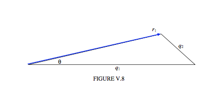
For a given mass ratio, the locus of r1 (the speed) versus θ (the scattering angle) is such that q1 and q2 are constant – in other words, it is a circle:
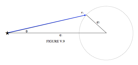
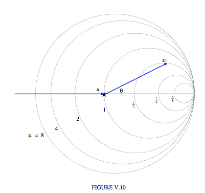
One can imagine that the first particle comes in from the left at speed u and the collision takes place at the asterisk, and, after collision, it is moving at a speed r1 times u in a direction θ, the magnitude of its velocity vector being determined by where the vector intersects the circle (in two possible places) given by Equation 5.5.24. The maximum scattering angle corresponds to a velocity vector that is tangent to the circle. If the asterisk is the pole (origin) of the polar coordinates, the centre of the circle is at a distance q1 from the pole, and its radius is q2. Figure V.10 shows the circles corresponding to several mass ratios. The Figure graphically illustrates the relation between u, v1, θ and μ. You can see, for example, that if μ>1, scattering through any angle is possible, and the relation between v1 and θ is unique; but if μ<1, only forward scattering is possible, up to a maximum θ, and, for a given θ, there are two solutions for v1.
This deals with what happens to the sphere m1. We can now turn our attention to m2. Starting from Equations 5.5.11, 5.5.12 and 5.5.13, we are going to want to eliminate r1 and θ - indeed anything that pertains to the sphere m1.
If you refer to Figure V.4 you will see that, after collision, m2 scoots off at an angle α1 to the original direction of motion of m1. Therefore I think it is of interest to find a relation between r2 (\dfrac{v_{2}}{u})and α1. If we succeed in doing this, it means that we can also find a relation, if we want it, between r2 and the impact parameter, since b′=sinα1. It is easy to eliminate r1 from Equations 5.5.12 and 5.5.13, and then you can get tan(θ+α1) from Equation 5.5.14, and hence get the required relation:
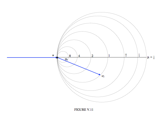
r2=2cosα11+μ.
I’ll draw this relation as a polar graph, r2 versus α1, in Figure V.11. I’ll leave the reader to work out and draw the relation between r2 and b′ if he or she wishes. Equation V.11 is the polar equation to a circle of radius 11+μ.
Suppose the mass ratio μ=m2m1=0.5 and the scattering angle is θ= 20°. Equation 5.5.16 or Figure V.10 will show that r1 = 0.8696 or 0.3833. Equation 5.5.17 will show that α1= 58° .4 or 11° .6 . And Equation 5.5.25 or Figure V.11 will show that r2 = 0.6983 or 1.306. I’ll leave it to the reader to determine which alternative values of r1, r2 and α1 go together.