
3.4: Geometrical Representations of Dynamical Motion


- Last updated
- Jul 3, 2021
- Save as PDF

( \newcommand{\kernel}{\mathrm{null}\,}\)
The powerful pattern-recognition capabilities of the human brain, coupled with geometrical representations of the motion of dynamical systems, provide a sensitive probe of periodic motion. The geometry of the motion often can provide more insight into the dynamics than inspection of mathematical functions. A system with n degrees of freedom is characterized by locations qi, velocities ˙qi, and momenta pi, in addition to the time t and instantaneous energy H(t). Geometrical representations of the dynamical correlations are illustrated by the configuration space and phase space representations of these 2n+2 variables.
Configuration space qi,qj,t
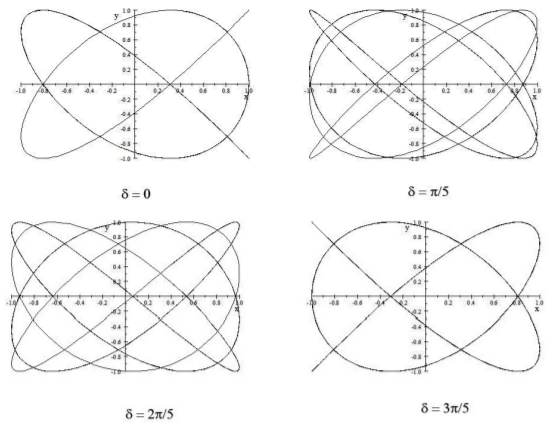
A configuration space plot shows the correlated motion of two spatial coordinates qi and qj averaged over time. An example is the two-dimensional linear oscillator with two equations of motion and solutions
m¨x+kxx=0m¨y+kyy=0
x(t)=Acos(ωxt)y(t)=Bcos(ωyt−δ)
where ω=√km. For unequal restoring force constants, kx≠ky the trajectory executes complicated Lissajous figures that depend on the angular frequencies ωx,ωy and the phase factor δ. When the ratio of the angular frequencies along the two axes is rational, that is ωxωy is a rational fraction, then the curve will repeat at regular intervals as shown in Figure 3.4.1, and this shape depends on the phase difference. Otherwise the trajectory gradually fills the whole rectangle.
State space, (qi,˙qi,t)
Visualization of a trajectory is enhanced by correlation of configuration qi and it’s corresponding velocity ˙qi which specifies the direction of the motion. The state space representation1 is especially valuable when discussing Lagrangian mechanics which is based on the Lagrangian L(q,˙q,t).
The free undamped harmonic oscillator provides a simple application of state space. Consider a mass m attached to a spring with linear spring constant k for which the equation of motion is
−kx=m¨x=m˙xd˙xdx
By integration this gives
12m˙x2+12kx2=E
The first term in Equation ??? is the kinetic energy, the second term is the potential energy, and E is the total energy which is conserved for this system. This equation can be expressed in terms of the state space coordinates as
˙x2(2Em)+x2(2Ek)=1
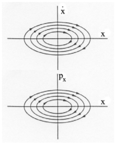
This corresponds to the equation of an ellipse for a state-space plot of ˙x versus x as shown in Figure 3.4.2-upper. The elliptical paths shown correspond to contours of constant total energy which is partitioned between kinetic and potential energy. For the coordinate axis shown, the motion of a representative point will be in a clockwise direction as the total oscillator energy is redistributed between potential to kinetic energy. The area of the ellipse is proportional to the total energy E.
Phase space, (qi,pi,t)
Phase space, which was introduced by J.W. Gibbs for the field of statistical mechanics, provides a fundamental graphical representation in classical mechanics. The phase space coordinates qipi are the conjugate coordinates (q,p) and are fundamental to Hamiltonian mechanics which is based on the Hamiltonian H(q,p,t). For a conservative system, only one phase-space curve passes through any point in phase space like the flow of an incompressible fluid. This makes phase space more useful than state space where many curves pass through any location. Lanczos [La49] defined an extended phase space using four-dimensional relativistic space-time as discussed in chapter 17.
Since px=m˙x for the non-relativistic, one-dimensional, linear oscillator, then Equation ??? can be rewritten in the form
p2x2mE+x2(2Ek)=1
This is the equation of an ellipse in the phase space diagram shown in Fig.3.4.2-lower which looks identical to Fig.3.4.2-upper since that the ordinate variable is multiplied by the constant m. That is, the only difference is the phase-space coordinates (x,px) replace the state-space coordinates (x,˙x). State space plots are used extensively in this chapter to describe oscillatory motion. Although phase space is more fundamental, both state space and phase space plots provide useful representations for characterizing and elucidating a wide variety of motion in classical mechanics. The following discussion of the undamped simple pendulum illustrates the general features of state space.
Plane pendulum
Consider a simple plane pendulum of mass m attached to a string of length l in a uniform gravitational field g. There is only one generalized coordinate, θ. Since the moment of inertia of the simple plane-pendulum is I=ml2 then the kinetic energy is
T=12ml2˙θ2
and the potential energy relative to the bottom dead center is
U=mgl(1−cosθ)
Thus the total energy equals
E=12ml2˙θ2+mgl(1−cosθ)=p2θ2ml2+mgl(1−cosθ)
where E is a constant of motion. Note that the angular momentum pθ is not a constant of motion since the angular acceleration ˙pθ explicitly depends on θ.
It is interesting to look at the solutions for the equation of motion for a plane pendulum on a (θ,˙θ) state space diagram shown in Figure 3.4.3. The curves shown are equally-spaced contours of constant total energy. Note that the trajectories are ellipses only at very small angles where 1−cosθ≈θ2, the contours are non-elliptical for higher amplitude oscillations. When the energy is in the range 0<E<2 mgl the motion corresponds to oscillations of the pendulum about θ=0. The center of the ellipse is at (0,0) which is a stable equilibrium point for the oscillation. However, when |E|>2mgl there is a phase change to rotational motion about the horizontal axis, that is, the pendulum swings around and over top dead center, i.e. it rotates continuously in one direction about the horizontal axis. The phase change occurs at E=2 mgl. and is designated by the separatrix trajectory.
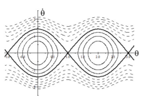
Figure 3.4.3 shows two cycles for θ to better illustrate the cyclic nature of the phase diagram. The closed loops, shown as fine solid lines, correspond to pendulum oscillations about θ=0 or 2π for E<2 mgl. The dashed lines show rolling motion for cases where the total energy E>2 mgl. The broad solid line is the separatrix that separates the rolling and oscillatory motion. Note that at the separatrix the kinetic energy and ˙θ are zero when the pendulum is at top dead center which occurs when θ=±π. The point (π,0) is an unstable equilibrium characterized by phase lines that are hyperbolic to this unstable equilibrium point. Note that θ=+π and −π correspond to the same physical point, that is, the phase diagram is better presented on a cylindrical phase space representation since θ is a cyclic variable that cycles around the cylinder whereas ˙θ oscillates equally about zero having both positive and negative values. The state-space diagram can be wrapped around a cylinder, then the unstable and stable equilibrium points will be at diametrically opposite locations on the surface of the cylinder at ˙θ=0. For small oscillations about equilibrium, also called librations, the correlation between ˙θ and θ is given by the clockwise closed loops wrapped on the cylindrical surface, whereas for energies |E|>2 mgl the positive ˙θ corresponds to counterclockwise rotations while the negative ˙θ corresponds to clockwise rotations.
State-space diagrams will be used for describing oscillatory motion in chapters 3 and 4. Phase space is used in statistical mechanics in order to handle the equations of motion for ensembles of ∼1023 independent particles since momentum is more fundamental than velocity. Rather than try to account separately for the motion of each particle for an ensemble, it is best to specify the region of phase space containing the ensemble. If the number of particles is conserved, then every point in the initial phase space must transform to corresponding points in the final phase space. This will be discussed in chapters 8.3 and 15.2.7.
1A universal name for the (q,˙q) representation has not been adopted in the literature. Therefore this book has adopted the name "state space". Lanczos [La49] uses the term "state space" to refer to the extended phase space (q,p,t) discussed in chapter 17.