3.10: Signal Processing
- Page ID
- 14011

\( \newcommand{\vecs}[1]{\overset { \scriptstyle \rightharpoonup} {\mathbf{#1}} } \)
\( \newcommand{\vecd}[1]{\overset{-\!-\!\rightharpoonup}{\vphantom{a}\smash {#1}}} \)
\( \newcommand{\dsum}{\displaystyle\sum\limits} \)
\( \newcommand{\dint}{\displaystyle\int\limits} \)
\( \newcommand{\dlim}{\displaystyle\lim\limits} \)
\( \newcommand{\id}{\mathrm{id}}\) \( \newcommand{\Span}{\mathrm{span}}\)
( \newcommand{\kernel}{\mathrm{null}\,}\) \( \newcommand{\range}{\mathrm{range}\,}\)
\( \newcommand{\RealPart}{\mathrm{Re}}\) \( \newcommand{\ImaginaryPart}{\mathrm{Im}}\)
\( \newcommand{\Argument}{\mathrm{Arg}}\) \( \newcommand{\norm}[1]{\| #1 \|}\)
\( \newcommand{\inner}[2]{\langle #1, #2 \rangle}\)
\( \newcommand{\Span}{\mathrm{span}}\)
\( \newcommand{\id}{\mathrm{id}}\)
\( \newcommand{\Span}{\mathrm{span}}\)
\( \newcommand{\kernel}{\mathrm{null}\,}\)
\( \newcommand{\range}{\mathrm{range}\,}\)
\( \newcommand{\RealPart}{\mathrm{Re}}\)
\( \newcommand{\ImaginaryPart}{\mathrm{Im}}\)
\( \newcommand{\Argument}{\mathrm{Arg}}\)
\( \newcommand{\norm}[1]{\| #1 \|}\)
\( \newcommand{\inner}[2]{\langle #1, #2 \rangle}\)
\( \newcommand{\Span}{\mathrm{span}}\) \( \newcommand{\AA}{\unicode[.8,0]{x212B}}\)
\( \newcommand{\vectorA}[1]{\vec{#1}} % arrow\)
\( \newcommand{\vectorAt}[1]{\vec{\text{#1}}} % arrow\)
\( \newcommand{\vectorB}[1]{\overset { \scriptstyle \rightharpoonup} {\mathbf{#1}} } \)
\( \newcommand{\vectorC}[1]{\textbf{#1}} \)
\( \newcommand{\vectorD}[1]{\overrightarrow{#1}} \)
\( \newcommand{\vectorDt}[1]{\overrightarrow{\text{#1}}} \)
\( \newcommand{\vectE}[1]{\overset{-\!-\!\rightharpoonup}{\vphantom{a}\smash{\mathbf {#1}}}} \)
\( \newcommand{\vecs}[1]{\overset { \scriptstyle \rightharpoonup} {\mathbf{#1}} } \)
\(\newcommand{\longvect}{\overrightarrow}\)
\( \newcommand{\vecd}[1]{\overset{-\!-\!\rightharpoonup}{\vphantom{a}\smash {#1}}} \)
\(\newcommand{\avec}{\mathbf a}\) \(\newcommand{\bvec}{\mathbf b}\) \(\newcommand{\cvec}{\mathbf c}\) \(\newcommand{\dvec}{\mathbf d}\) \(\newcommand{\dtil}{\widetilde{\mathbf d}}\) \(\newcommand{\evec}{\mathbf e}\) \(\newcommand{\fvec}{\mathbf f}\) \(\newcommand{\nvec}{\mathbf n}\) \(\newcommand{\pvec}{\mathbf p}\) \(\newcommand{\qvec}{\mathbf q}\) \(\newcommand{\svec}{\mathbf s}\) \(\newcommand{\tvec}{\mathbf t}\) \(\newcommand{\uvec}{\mathbf u}\) \(\newcommand{\vvec}{\mathbf v}\) \(\newcommand{\wvec}{\mathbf w}\) \(\newcommand{\xvec}{\mathbf x}\) \(\newcommand{\yvec}{\mathbf y}\) \(\newcommand{\zvec}{\mathbf z}\) \(\newcommand{\rvec}{\mathbf r}\) \(\newcommand{\mvec}{\mathbf m}\) \(\newcommand{\zerovec}{\mathbf 0}\) \(\newcommand{\onevec}{\mathbf 1}\) \(\newcommand{\real}{\mathbb R}\) \(\newcommand{\twovec}[2]{\left[\begin{array}{r}#1 \\ #2 \end{array}\right]}\) \(\newcommand{\ctwovec}[2]{\left[\begin{array}{c}#1 \\ #2 \end{array}\right]}\) \(\newcommand{\threevec}[3]{\left[\begin{array}{r}#1 \\ #2 \\ #3 \end{array}\right]}\) \(\newcommand{\cthreevec}[3]{\left[\begin{array}{c}#1 \\ #2 \\ #3 \end{array}\right]}\) \(\newcommand{\fourvec}[4]{\left[\begin{array}{r}#1 \\ #2 \\ #3 \\ #4 \end{array}\right]}\) \(\newcommand{\cfourvec}[4]{\left[\begin{array}{c}#1 \\ #2 \\ #3 \\ #4 \end{array}\right]}\) \(\newcommand{\fivevec}[5]{\left[\begin{array}{r}#1 \\ #2 \\ #3 \\ #4 \\ #5 \\ \end{array}\right]}\) \(\newcommand{\cfivevec}[5]{\left[\begin{array}{c}#1 \\ #2 \\ #3 \\ #4 \\ #5 \\ \end{array}\right]}\) \(\newcommand{\mattwo}[4]{\left[\begin{array}{rr}#1 \amp #2 \\ #3 \amp #4 \\ \end{array}\right]}\) \(\newcommand{\laspan}[1]{\text{Span}\{#1\}}\) \(\newcommand{\bcal}{\cal B}\) \(\newcommand{\ccal}{\cal C}\) \(\newcommand{\scal}{\cal S}\) \(\newcommand{\wcal}{\cal W}\) \(\newcommand{\ecal}{\cal E}\) \(\newcommand{\coords}[2]{\left\{#1\right\}_{#2}}\) \(\newcommand{\gray}[1]{\color{gray}{#1}}\) \(\newcommand{\lgray}[1]{\color{lightgray}{#1}}\) \(\newcommand{\rank}{\operatorname{rank}}\) \(\newcommand{\row}{\text{Row}}\) \(\newcommand{\col}{\text{Col}}\) \(\renewcommand{\row}{\text{Row}}\) \(\newcommand{\nul}{\text{Nul}}\) \(\newcommand{\var}{\text{Var}}\) \(\newcommand{\corr}{\text{corr}}\) \(\newcommand{\len}[1]{\left|#1\right|}\) \(\newcommand{\bbar}{\overline{\bvec}}\) \(\newcommand{\bhat}{\widehat{\bvec}}\) \(\newcommand{\bperp}{\bvec^\perp}\) \(\newcommand{\xhat}{\widehat{\xvec}}\) \(\newcommand{\vhat}{\widehat{\vvec}}\) \(\newcommand{\uhat}{\widehat{\uvec}}\) \(\newcommand{\what}{\widehat{\wvec}}\) \(\newcommand{\Sighat}{\widehat{\Sigma}}\) \(\newcommand{\lt}{<}\) \(\newcommand{\gt}{>}\) \(\newcommand{\amp}{&}\) \(\definecolor{fillinmathshade}{gray}{0.9}\)It has been shown that the response of the linearly-damped linear oscillator, subject to any arbitrary periodic force, can be calculated using a frequency decomposition, (Fourier analysis), of the force, appendix \(19.9\). The response can equally well can be calculated using a time-ordered discrete-time sampling of the pulse shape; that is, the Green’s function approach, appendix \(19.9\). The linearly-damped, linear oscillator is the simplest example of a linear system that exhibits both resonance and frequency-dependent response. Typical physical linear systems exhibit far more complicated response functions with multiple resonances and corresponding frequency response. For example, an automobile suspension system involves four wheels and associated springs plus dampers allowing the car to rock sideways, or forward and backward, in addition to the updown motion, when subject to the forces produced by a rough road. Similarly a suspension bridge or aircraft wing can twist as well as bend due to air turbulence, or a building can undergo complicated oscillations due to seismic waves. An acoustic system exhibits similar complexity. Signal analysis and signal processing is of pivotal importance to elucidating the response of complicated linear systems to complicated periodic forcing functions. This is used extensively in engineering, acoustics, and science.
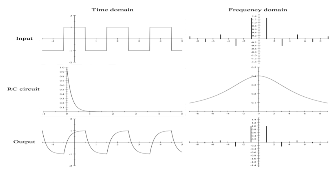
The response of a low-pass filter, such as an R-C circuit or a coaxial cable, to a input square wave, shown in Figure \(\PageIndex{1}\), provides a simple example of the relative advantages of using the complementary Fourier analysis in the frequency domain, or the Green’s discrete-function analysis in the time domain. The response of a repetitive square-wave input signal is shown in the time domain and the Fourier transform to the frequency domain. The middle curves show the time dependence for the response of the low-pass filter to an impulse \(I(t)\) and the Fourier transform \(H(\omega)\). The output of the low-pass filter can be calculated by folding the input square wave and impulse time dependence in the time domain as shown on the left or by folding of their Fourier transforms shown on the right. Working in the frequency domain the response of linear mechanical systems, such as an automobile suspension or a musical instrument, as well as linear electronic signal processing systems such as amplifiers, loudspeakers and microphones, can be treated as black boxes having a certain transfer function \(H(\omega, \phi)\) describing the gain and phase shift versus frequency. That is, the output wave frequency decomposition is
\[G(\omega)_{output} = H(\omega , \phi) \cdot G(\omega)_{input} \label{3.111}\]
Working in the time domain, the the low-pass system has an impulse response \(I(t) = e^{-\frac{t}{\tau}}\), which is the Fourier transform of the transfer function \(H(\omega , \phi ) \). In the time domain
\[y(t)_{output} = \int^{\infty}_{-\infty} x(\tau ) \cdot I(t - \tau) d \tau \label{3.112} \]
This is shown schematically in Figure \(\PageIndex{1}\). The Fourier transformation connects the three quantities in the time domain with the corresponding three in the frequency domain. For example, the impulse response of the low-pass filter has a fall time of \(\tau\) which is related by a Fourier transform to the width of the transfer function. Thus the time and frequency domain approaches are closely related and give the same result for the output signal for the low-pass filter to the applied square-wave input signal. The result is that the higher-frequency components are attenuated leading to slow rise and fall times in the time domain.
Analog signal processing and Fourier analysis were the primary tools to analyze and process all forms of periodic motion during the 20\(^{th}\) century. For example, musical instruments, mechanical systems, electronic circuits, all employed resonant systems to enhance the desired frequencies and suppress the undesirable frequencies and the signals were observed using analog oscilloscopes. The remarkable development of computing has enabled use of digital signal processing leading to a revolution in signal processing that has had a profound impact on both science and engineering. For example, the digital oscilloscope, which can sample at frequencies above \(10^9\) \(Hz\) has replaced the analog oscilloscope because it allows sophisticated analysis of each individual signal that was not possible using analog signal processing. For example, the analog approach in nuclear physics involved tiny analog electric signals, produced by many individual radiation detectors, that were transmitted hundreds of meters via carefully shielded and expensive coaxial cables to the data room where the signals were amplified and signal processed using analog filters to maximize the signal to noise in order to separate the signal from the background noise. Stray electromagnetic radiation picked up via the cables significantly degraded the signals. The performance and limitations of the analog electronics severely restricted the pulse processing capabilities. Digital signal processing has rapidly replaced analog signal processing. Analog to digital detector circuits are built directly into the electronics for each individual detector so that only digital information needs to be transmitted from each detector to the analysis computers. Computer processing provides unlimited and flexible processing capabilities for the digital signals greatly enhancing the response and sensitivity of our detector systems. Common examples of digital signal processing are digital CD and DVD disks.