3.9: Waveform Analysis

Harmonic decomposition

As described in appendix $19.9$, when superposition applies, then a Fourier series decomposition of the form $\ref{eq:3.101}$ can be made of any periodic function where

$$\label{eq:3.101} F(t) = \sum_{n=1}^{N} \alpha_n \cos(n\omega_0t + \phi_n )$$

or the more general Fourier Transform can be made for an aperiodic function where

$$\label{eq:3.102} F(t) = \int \alpha (\omega) \cos(\omega t + \phi(\omega)) dt$$

Any linear system that is subject to the forcing function $F(t)$ has an output that can be expressed as a linear superposition of the solutions of the individual harmonic components of the forcing function. Fourier analysis of periodic waveforms in terms of harmonic trigonometric functions plays a key role in describing oscillatory motion in classical mechanics and signal processing for linear systems. Fourier’s theorem states that any arbitrary forcing function $F(t)$ can be decomposed into a sum of harmonic terms. As a consequence two equivalent representations can be used to describe signals and waves; the first is in the time domain which describes the time dependence of the signal. The second is in the frequency domain which describes the frequency decomposition of the signal. Fourier analysis relates these equivalent representations.

Figure $\PageIndex{1}$: The time and frequency representations of a system exhibiting beats.

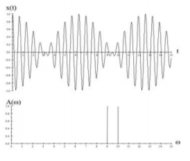
For example, the superposition of two equal intensity harmonic oscillators in the time domain is given by

$$\label{eq:3.103} y(t) = A\cos(\omega_1t) + A\cos(\omega_2t) \\ = 2A\cos \Bigg [ \Bigg ( \frac{\omega_1 + \omega_2}{2} \Bigg ) t \Bigg] \cos \Bigg [ \Bigg (\frac{\omega_1 - \omega_2}{2} \Bigg ) t \Bigg ]$$

The free linearly-damped linear oscillator

The response of the free, linearly-damped, linear oscillator is one of the most frequently encountered waveforms in science and thus it is useful to investigate the Fourier transform of this waveform. The damped waveform for the underdamped case, shown in figure (3.5.1) is given by equation (3.5.12), that is

$$\begin{align} \label{eq:3.104} f(t) & = & Ae^{-\frac{\Gamma}{2}t}\cos(\omega_1t-\delta) && t \geq 0 \\ \label{eq:3.105} f(t) & = & 0 && t < 0 \end{align}$$

where $\omega_1^2 = \omega_0^2 - \big ( \frac{\Gamma}{2} \big )^2$ and where $\omega_0$ is the angular frequency of the underdamped system. The Fourier transform is given by

$$\label{eq:3.106} G(\omega) = \frac{\omega_0}{(\omega^2 - \omega_1^2)^2 + (\Gamma \omega)^2} [ (\omega^2 - \omega_1^2) - i \Gamma \omega ]$$

which is complex and has the famous Lorentz form.

Figure $\PageIndex{2}$: The intensity $f(t)^2$ and Fourier transform $|G(w)|^2$ of the free linearly-underdamped harmonic oscillator with $\omega_0 = 10$ and damping $\Gamma = 1$.

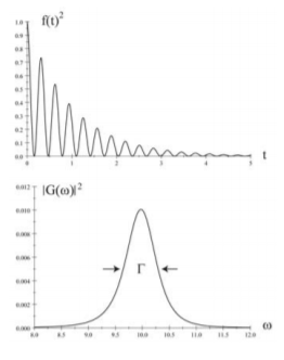
The intensity of the wave gives

$$|f(t)|^2 = A^2 e^{-\Gamma t} \cos^2 (\omega_1 t - \delta) \label{3.107}$$

$$|G ( \omega)|^2 = \frac{\omega^2_0}{(\omega^2 - \omega^2_1)^2 + ( \Gamma \omega )^2} \label{3.108}$$

Note that since the average over $2\pi$ of $\cos^2 = \frac{1}{2}$, then the average over the $\cos^2 (\omega_1 t − \delta)$ term gives the intensity $I(t) = \frac{A^2}{2} e^{−\Gamma t}$ which has a mean lifetime for the decay of $\tau = \frac{1}{\Gamma}$. The $|G (\omega )|^2$ distribution has the classic Lorentzian shape, shown in Figure $\PageIndex{2}$, which has a full width at half-maximum, FWHM, equal to $\Gamma$. Note that $G (\omega )$ is complex and thus one also can determine the phase shift $\delta$ which is given by the ratio of the imaginary to real parts of Equation $\ref{eq:3.105}$, i.e. $\tan \delta = \frac{\Gamma\omega}{ (\omega^2−\omega^2_1)}$.

The mean lifetime of the exponential decay of the intensity can be determined either by measuring $\tau$ from the time dependence, or measuring the FWHM $\Gamma = \frac{1}{\tau}$ of the Fourier transform $|G (\omega )|^2$. In nuclear and atomic physics excited levels decay by photon emission with the wave form of the free linearly-damped, linear oscillator. Typically the mean lifetime $\tau$ usually can be measured when $\tau \gtrsim 10^{−12} s$ whereas for shorter lifetimes the radiation width $\Gamma$ becomes sufficiently large to be measured. Thus the two experimental approaches are complementary.

Damped linear oscillator subject to an arbitrary periodic force

Fourier’s theorem states that any arbitrary forcing function $F(t)$ can be decomposed into a sum of harmonic terms. Consider the response of a damped linear oscillator to an arbitrary periodic force.

$$F(t) = \sum^{N}_{n=0} \alpha_n F_0 ( \omega_n) \cos (\omega_n t + \delta_n) \label{3.109}$$

For each harmonic term $\omega_n$ the response of a linearly-damped linear oscillator to the forcing function $F(t) = F_0 (\omega) \cos ( \omega_n t)$ is given by equation (3.6.18-3.6.20) to be

$$\begin{align} x(t)_{Total} & = & x(t)_T + x(t)_S \nonumber \\ & = & \frac{F_0 (\omega_n)}{m} \left[ e^{-\frac{\Gamma}{2}t} \cos (\omega_1 t - \delta_n) + \frac{1}{\sqrt{ (\omega^2_0 - \omega^2_n)^2 + (\Gamma \omega_n)^2}} \cos (\omega_n t - \delta_n) \right] \label{3.110} \end{align}$$

The amplitude is obtained by substituting into Equation $\ref{3.110}$ the derived values $\frac{F_0 (\omega_n)}{m}$ from the Fourier analysis.

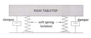
Example $\PageIndex{1}$: Vibration isolation

Frequently it is desired to isolate instrumentation from the influence of horizontal and vertical external vibrations that exist in its environment. One arrangement to achieve this isolation is to mount a heavy base of mass $m$ on weak springs of spring constant $k$ plus weak damping. The response of this system is given by Equation $\ref{3.109}$ which exhibits a resonance at the angular frequency $\omega^2_R = \omega^2_0 − 2 ( \frac{\Gamma}{2})^2$ associated with each resonant frequency $\omega_0$ of the system. For each resonant frequency the system amplifies the vibrational amplitude for angular frequencies close to resonance that is, below $\sqrt{2} \omega_0$, while it attenuates the vibration roughly by a factor of $(\frac{\omega_0}{\omega})^2$ at higher frequencies. To avoid the amplification near the resonance it is necessary to make $\omega_0$ very much smaller than the frequency range of the vibrational spectrum and have a moderately high $Q$ value. This is achieved by use a very heavy base and weak spring constant so that $\omega_0$ is very small. A typical table may have the resonance frequency at 0.5 $Hz$ which is well below typical perturbing vibrational frequencies, and thus the table attenuates the vibration by 99% at 5 $Hz$ and even more attenuation for higher frequency perturbations. This principle is used extensively in design of vibration-isolation tables for optics or microbalance equipment.

Figure $\PageIndex{3}$: Seismic isolation of an optical bench.