25.2: Planetary Orbits

We now commence a study of the Kepler Problem. We shall determine the equation of motion for the motions of two bodies interacting via a gravitational force (two-body problem) using both force methods and conservation laws.

Reducing the Two-Body Problem into a One-Body Problem

We shall begin by showing how the motion of two bodies interacting via a gravitational force (two-body problem) is mathematically equivalent to the motion of a single body acted on by an external central gravitational force, where the mass of the single body is the reduced mass \(\mu\),

\[\frac{1}{\mu}=\frac{1}{m_{1}}+\frac{1}{m_{2}} \Rightarrow \mu=\frac{m_{1} m_{2}}{m_{1}+m_{2}} \nonumber \]

Once we solve for the motion of the reduced body in this equivalent one-body problem, we can then return to the real two-body problem and solve for the actual motion of the two original bodies. The reduced mass was introduced in Chapter 13 Appendix A of these notes. That appendix used similar but slightly different notation from that used in this chapter.

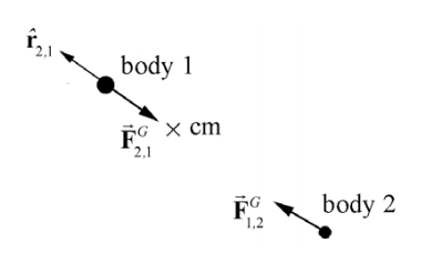
Consider the gravitational interaction between two bodies with masses m and as 1 m2 shown in Figure 25.1.

Figure 25.1 Gravitational force between two bodies

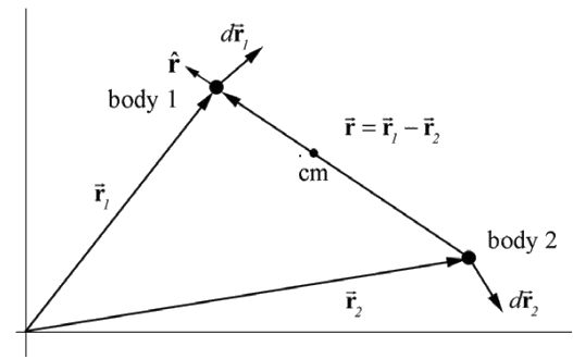
Choose a coordinate system with a choice of origin such that body 1 has position \(\overrightarrow{\mathbf{r}}_{1}\) and body 2 has position \(\overrightarrow{\mathbf{r}}_{2}\) (Figure 25.2). The relative position vector \(\overrightarrow{\mathbf{r}}\) pointing from body 2 to body 1 is \(\overrightarrow{\mathbf{r}}=\overrightarrow{\mathbf{r}}_{1}-\overrightarrow{\mathbf{r}}_{2}\) We denote the magnitude of \(\overrightarrow{\mathbf{r}} \text { by }|\overrightarrow{\mathbf{r}}|=r\), where r is the distance between the bodies, and \(\hat{\mathbf{r}}\) is the unit vector pointing from body 2 to body 1, so that \(\overrightarrow{\mathbf{r}}=r \hat{\mathbf{r}}\).

Figure 25.2 Coordinate system for the two-body problem

The force on body 1 (due to the interaction of the two bodies) can be described by Newton’s Universal Law of Gravitation

\[\overrightarrow{\mathbf{F}}_{2,1}=-F_{2,1} \hat{\mathbf{r}}=-G \frac{m_{1} m_{2}}{r^{2}} \hat{\mathbf{r}} \nonumber \]

Recall that Newton’s Third Law requires that the force on body 2 is equal in magnitude and opposite in direction to the force on body 1,

\[\overrightarrow{\mathbf{F}}_{1,2}=-\overrightarrow{\mathbf{F}}_{2,1} \nonumber \]

Newton’s Second Law can be applied individually to the two bodies:

\[\begin{array}{l}
\overrightarrow{\mathbf{F}}_{2,1}=m_{1} \frac{d^{2} \overrightarrow{\mathbf{r}}_{1}}{d t^{2}} \\
\overrightarrow{\mathbf{F}}_{1,2}=m_{2} \frac{d^{2} \overrightarrow{\mathbf{r}}_{2}}{d t^{2}}
\end{array} \nonumber \]

Dividing through by the mass in each of Equations (25.2.4) and (25.2.5) yields

\[\frac{\overrightarrow{\mathbf{F}}_{2,1}}{m_{1}}=\frac{d^{2} \overrightarrow{\mathbf{r}}_{1}}{d t^{2}} \nonumber \]

\[\frac{\overrightarrow{\mathbf{F}}_{1,2}}{m_{2}}=\frac{d^{2} \overrightarrow{\mathbf{r}}_{2}}{d t^{2}} \nonumber \]

Subtracting the expression in Equation (25.2.7) from that in Equation (25.2.6) yields

\[\frac{\overrightarrow{\mathbf{F}}_{2,1}}{m_{1}}-\frac{\overrightarrow{\mathbf{F}}_{1,2}}{m_{2}}=\frac{d^{2} \overrightarrow{\mathbf{r}}_{1}}{d t^{2}}-\frac{d^{2} \overrightarrow{\mathbf{r}}_{2}}{d t^{2}}=\frac{d^{2} \overrightarrow{\mathbf{r}}}{d t^{2}} \nonumber \]

Using Newton’s Third Law, Equation (25.2.3), Equation (25.2.8) becomes

\[\overrightarrow{\mathbf{F}}_{2,1}\left(\frac{1}{m_{1}}+\frac{1}{m_{2}}\right)=\frac{d^{2} \overrightarrow{\mathbf{r}}}{d t^{2}} \nonumber \]

Using the reduced mass µ , as defined in Equation (25.2.1), Equation (25.2.9) becomes

\[\begin{array}{l}
\frac{\overrightarrow{\mathbf{F}}_{2,1}}{\mu}=\frac{d^{2} \overrightarrow{\mathbf{r}}}{d t^{2}} \\
\overrightarrow{\mathbf{F}}_{2,1}=\mu \frac{d^{2} \overrightarrow{\mathbf{r}}}{d t^{2}}
\end{array} \nonumber \]

where \(\overrightarrow{\mathbf{F}}_{2,1}\) is given by Equation (25.2.2).

Our result has a special interpretation using Newton’s Second Law. Let \(\mu\) be the mass of a single body with position vector \(\overrightarrow{\mathbf{r}}=r \hat{\mathbf{r}}\) with respect to an origin O , where \(\hat{\mathbf{r}}\) is the unit vector pointing from the origin O to the single body. Then the equation of motion, Equation (25.2.10), implies that the single body of mass \(\mu\) is under the influence of an attractive gravitational force pointing toward the origin. So, the original two-body gravitational problem has now been reduced to an equivalent one-body problem, involving a single body with mass \(\mu\) under the influence of a central force \(\overrightarrow{\mathbf{F}}^{G}=-\mathrm{F}_{2,1} \hat{\mathbf{r}}\) Note that in this reformulation, there is no body located at the central point (the origin O ). The parameter r in the two-body problem is the relative distance between the original two bodies, while the same parameter r in the one-body problem is the distance between the single body and the central point. This reduction generalizes to all central forces.