2.5: Plane Laminas and Mass Points distributed in a Plane

In Figure II.6a, the two unbroken lines represent two fixed coordinate axes. I have drawn several point masses $m_{1}, m_{2}, m_{3}$ distributed in a plane.

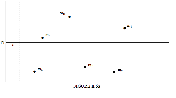
The $x$-coordinate of mass $m_{i}$ is $x_{i}$. The dashed line is moveable, and it $x$-coordinate is $x$, so that the distance of $m_{i}$ this line is $x_{i} -x$ The moment of inertia of the system of masses about the dashed line is

$$\begin{equation} \ I = m_{1}(x_{1}-x)^{2} + m_{2}(x_{2}-x)^{2}+ m_{3}(x_{3}-x)^{2} + ... . \tag{2.5.1}\label{eq:2.5.1} \end{equation}$$

Now imagine what happens if the dashed line is moved to the right. The moment of inertia decreases – and decreases - and decreases. But eventually the line finds itself to the right of $m_{4}$, and then of $m_{5}$, and then of $m_{6}$. After that is by no means obvious that the moment of inertia is going to continue to decrease. Indeed, by this time it is clear that at some point $I$ is going to go through a minimum and then start to increase again as more and more of the masses find themselves to the left of the dashed line. Just where is the dashed line when the moment of inertia is a minimum? I’ll leave you to differentiate Equation $\ref{eq:2.5.1}$ with respect to $x$, and hence show that $I$ is least when

$$x = \frac{m_{1}x_{1} +m_{2}x_{2} + m_{3}x_{3}+ ...}{m_{1} +m_{2} + m_{3}+ ...} \tag{2.5.2}\label{eq:2.5.2}$$

That is, the moment of inertia is least when $\overline{x} = x$. That is, the moment of inertia is least for an axis passing through the centre of mass.

In Figure II.6b, the line CC passes through the centre of mass; the moment of inertia is least about this line. The line AA is at a distance $\overline{x}$ from CC, and the moment of inertia is greater about AA than about CC. The Parallel Axes Theorem tells us by how much.

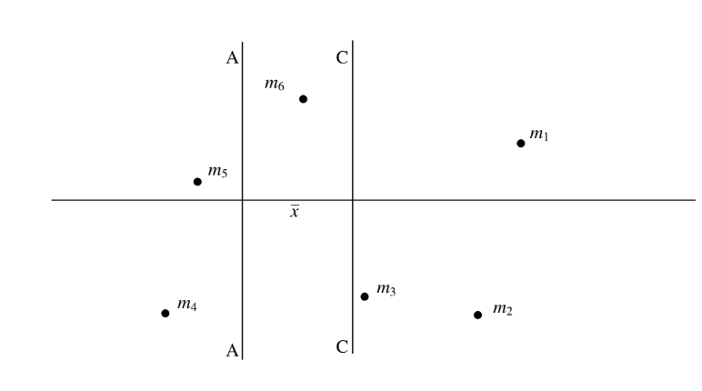
Let us measure distances from CC, so that the distance of $m_{i}$ from CC is $x_{i}$ and the distance of $m_{i}$ from AA is $x_{i} + \overline{x}$.

It is clear that $I_{CC} = \sum m_{i}x^{2}_{i}$

and that

$$I_{AA} = \sum m_{i} (x_{i} + \overline{x})^{2} = \sum m_{i}x^{2}_{i} + 2\overline{x} \sum m_{i}x_{i} + \overline{x}^{2} \sum m_{i}. \tag{2.5.3}\label{eq:2.5.3}$$

The first term on the right hand side is $I_{CC}$. The sum in the second term is the first moment of mass about the centre of mass, and is zero. The sum in the third term is the total mass. We therefore arrive at the Parallel Axes Theorem.

$$I_{AA}=I_{CC} +M\overline{x}^{2}. \tag{2.5.4}\label{eq:2.54}$$

In words, the moment of inertia about an arbitrary axis is equal to the moment of inertia about a parallel axis through the centre of mass plus the total mass times the square of the distance between the parallel axes. The theorem holds also for masses distributed in three-dimensional space.

The Perpendicular Axes Theorem, on the other hand, holds only for masses distributed in a plane, or for plane laminas.

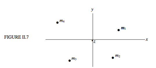
Figure II.7 shows some point masses distributed in the $xy$ plane, the $z$ axis being perpendicular to the plane of the paper. The moments of inertia about the $x , y$ and $z$ axes are denoted respectively by $A, B$ and $C$. The distance of $m_{i}$ from the $z$ axis is $(x^{2}_{i} + y^{2}_{i})^\frac{1}{2}$Therefore the moment of inertia of the masses about the z axis is

$$C = \sum m_{i} (x^{2}_{i} + y^{2}_{i}) \tag{2.5.5}\label{eq:2.5.5}$$

That is to say:

$$C = A + B \tag{2.5.6}\label{eq:2.5.6}$$

This is the Perpendicular Axes Theorem. Note again very carefully that, unlike the parallel axes theorem, this theorem applies only to plane laminas and to point masses distributed in a plane.

Examples of the Use of the Parallel and Perpendicular Axes Theorems.

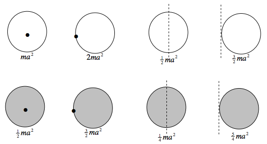
From Section 2.3 we know the moments of inertia of discs, rods and triangular laminas. We can make use of the parallel and perpendicular axes theorems to write down the moments of inertia of most of the following examples almost by sight, with no calculus.

Hoop and discs, radius $a$.

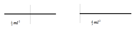
Rods, length $2l$.

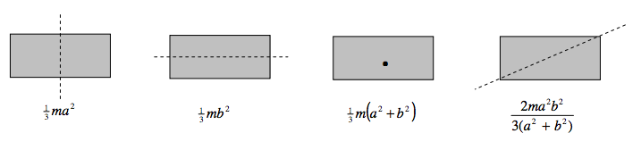
Rectangular laminas, sides $2a$ and $2b$; $a > b$.

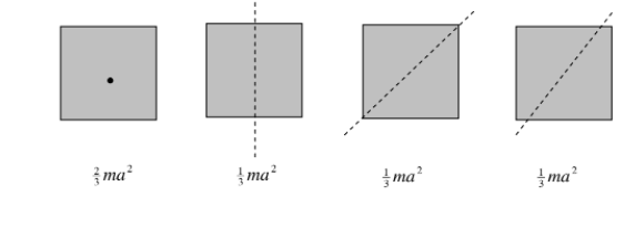
Square laminas, side $2a$.

Triangular laminas.

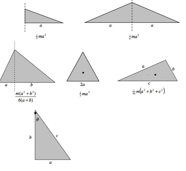
$I = \frac{1}{6} ma^{2} (1+3cot^{2} \theta) = \frac{1}{6}mb^{2} (3 + tan^2 \theta) = \frac{1}{6}mc^{2}(3-2sin^2\theta)$

$=\frac{1}{6}m(2b^2+ c^2) = \frac{1}{6} m(3c^2-2a^2) = \frac{1}{6} m(a^3b^2)$