
17.12: A Driven System
- Page ID
- 8506

\( \newcommand{\vecs}[1]{\overset { \scriptstyle \rightharpoonup} {\mathbf{#1}} } \)
\( \newcommand{\vecd}[1]{\overset{-\!-\!\rightharpoonup}{\vphantom{a}\smash {#1}}} \)
\( \newcommand{\dsum}{\displaystyle\sum\limits} \)
\( \newcommand{\dint}{\displaystyle\int\limits} \)
\( \newcommand{\dlim}{\displaystyle\lim\limits} \)
\( \newcommand{\id}{\mathrm{id}}\) \( \newcommand{\Span}{\mathrm{span}}\)
( \newcommand{\kernel}{\mathrm{null}\,}\) \( \newcommand{\range}{\mathrm{range}\,}\)
\( \newcommand{\RealPart}{\mathrm{Re}}\) \( \newcommand{\ImaginaryPart}{\mathrm{Im}}\)
\( \newcommand{\Argument}{\mathrm{Arg}}\) \( \newcommand{\norm}[1]{\| #1 \|}\)
\( \newcommand{\inner}[2]{\langle #1, #2 \rangle}\)
\( \newcommand{\Span}{\mathrm{span}}\)
\( \newcommand{\id}{\mathrm{id}}\)
\( \newcommand{\Span}{\mathrm{span}}\)
\( \newcommand{\kernel}{\mathrm{null}\,}\)
\( \newcommand{\range}{\mathrm{range}\,}\)
\( \newcommand{\RealPart}{\mathrm{Re}}\)
\( \newcommand{\ImaginaryPart}{\mathrm{Im}}\)
\( \newcommand{\Argument}{\mathrm{Arg}}\)
\( \newcommand{\norm}[1]{\| #1 \|}\)
\( \newcommand{\inner}[2]{\langle #1, #2 \rangle}\)
\( \newcommand{\Span}{\mathrm{span}}\) \( \newcommand{\AA}{\unicode[.8,0]{x212B}}\)
\( \newcommand{\vectorA}[1]{\vec{#1}} % arrow\)
\( \newcommand{\vectorAt}[1]{\vec{\text{#1}}} % arrow\)
\( \newcommand{\vectorB}[1]{\overset { \scriptstyle \rightharpoonup} {\mathbf{#1}} } \)
\( \newcommand{\vectorC}[1]{\textbf{#1}} \)
\( \newcommand{\vectorD}[1]{\overrightarrow{#1}} \)
\( \newcommand{\vectorDt}[1]{\overrightarrow{\text{#1}}} \)
\( \newcommand{\vectE}[1]{\overset{-\!-\!\rightharpoonup}{\vphantom{a}\smash{\mathbf {#1}}}} \)
\( \newcommand{\vecs}[1]{\overset { \scriptstyle \rightharpoonup} {\mathbf{#1}} } \)
\(\newcommand{\longvect}{\overrightarrow}\)
\( \newcommand{\vecd}[1]{\overset{-\!-\!\rightharpoonup}{\vphantom{a}\smash {#1}}} \)
\(\newcommand{\avec}{\mathbf a}\) \(\newcommand{\bvec}{\mathbf b}\) \(\newcommand{\cvec}{\mathbf c}\) \(\newcommand{\dvec}{\mathbf d}\) \(\newcommand{\dtil}{\widetilde{\mathbf d}}\) \(\newcommand{\evec}{\mathbf e}\) \(\newcommand{\fvec}{\mathbf f}\) \(\newcommand{\nvec}{\mathbf n}\) \(\newcommand{\pvec}{\mathbf p}\) \(\newcommand{\qvec}{\mathbf q}\) \(\newcommand{\svec}{\mathbf s}\) \(\newcommand{\tvec}{\mathbf t}\) \(\newcommand{\uvec}{\mathbf u}\) \(\newcommand{\vvec}{\mathbf v}\) \(\newcommand{\wvec}{\mathbf w}\) \(\newcommand{\xvec}{\mathbf x}\) \(\newcommand{\yvec}{\mathbf y}\) \(\newcommand{\zvec}{\mathbf z}\) \(\newcommand{\rvec}{\mathbf r}\) \(\newcommand{\mvec}{\mathbf m}\) \(\newcommand{\zerovec}{\mathbf 0}\) \(\newcommand{\onevec}{\mathbf 1}\) \(\newcommand{\real}{\mathbb R}\) \(\newcommand{\twovec}[2]{\left[\begin{array}{r}#1 \\ #2 \end{array}\right]}\) \(\newcommand{\ctwovec}[2]{\left[\begin{array}{c}#1 \\ #2 \end{array}\right]}\) \(\newcommand{\threevec}[3]{\left[\begin{array}{r}#1 \\ #2 \\ #3 \end{array}\right]}\) \(\newcommand{\cthreevec}[3]{\left[\begin{array}{c}#1 \\ #2 \\ #3 \end{array}\right]}\) \(\newcommand{\fourvec}[4]{\left[\begin{array}{r}#1 \\ #2 \\ #3 \\ #4 \end{array}\right]}\) \(\newcommand{\cfourvec}[4]{\left[\begin{array}{c}#1 \\ #2 \\ #3 \\ #4 \end{array}\right]}\) \(\newcommand{\fivevec}[5]{\left[\begin{array}{r}#1 \\ #2 \\ #3 \\ #4 \\ #5 \\ \end{array}\right]}\) \(\newcommand{\cfivevec}[5]{\left[\begin{array}{c}#1 \\ #2 \\ #3 \\ #4 \\ #5 \\ \end{array}\right]}\) \(\newcommand{\mattwo}[4]{\left[\begin{array}{rr}#1 \amp #2 \\ #3 \amp #4 \\ \end{array}\right]}\) \(\newcommand{\laspan}[1]{\text{Span}\{#1\}}\) \(\newcommand{\bcal}{\cal B}\) \(\newcommand{\ccal}{\cal C}\) \(\newcommand{\scal}{\cal S}\) \(\newcommand{\wcal}{\cal W}\) \(\newcommand{\ecal}{\cal E}\) \(\newcommand{\coords}[2]{\left\{#1\right\}_{#2}}\) \(\newcommand{\gray}[1]{\color{gray}{#1}}\) \(\newcommand{\lgray}[1]{\color{lightgray}{#1}}\) \(\newcommand{\rank}{\operatorname{rank}}\) \(\newcommand{\row}{\text{Row}}\) \(\newcommand{\col}{\text{Col}}\) \(\renewcommand{\row}{\text{Row}}\) \(\newcommand{\nul}{\text{Nul}}\) \(\newcommand{\var}{\text{Var}}\) \(\newcommand{\corr}{\text{corr}}\) \(\newcommand{\len}[1]{\left|#1\right|}\) \(\newcommand{\bbar}{\overline{\bvec}}\) \(\newcommand{\bhat}{\widehat{\bvec}}\) \(\newcommand{\bperp}{\bvec^\perp}\) \(\newcommand{\xhat}{\widehat{\xvec}}\) \(\newcommand{\vhat}{\widehat{\vvec}}\) \(\newcommand{\uhat}{\widehat{\uvec}}\) \(\newcommand{\what}{\widehat{\wvec}}\) \(\newcommand{\Sighat}{\widehat{\Sigma}}\) \(\newcommand{\lt}{<}\) \(\newcommand{\gt}{>}\) \(\newcommand{\amp}{&}\) \(\definecolor{fillinmathshade}{gray}{0.9}\)It would probably be useful before reading this and the next section to review Chapters 11 and 12.
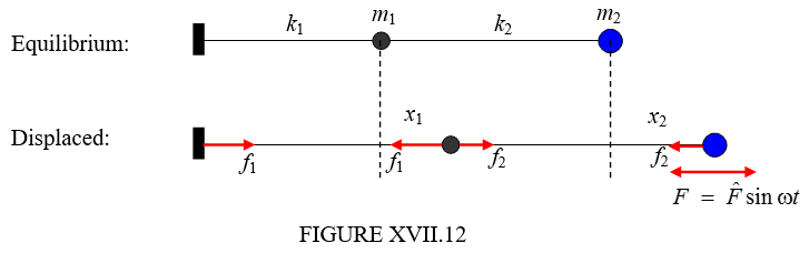
Figure XVII.12 shows the same system as figure XVII.2, except that, instead of being left to vibrate on its own, the second mass is subject to a periodic force \( F\ =\ \hat{F}\sin\omega t\). For the time being, we’ll suppose that there is no damping. Either way, it is not a conservative force, and Lagrange’s equation will be used in the form of Equation 13.4.12. As in Section 17.2, the kinetic energy is
\[ T =\frac{1}{2}m_{1}\dot{x}_{1}^{2}\ +\ \frac{1}{2}m_{2}\dot{x}_{2}^{2}\label{17.12.1} \]
Lagrange’s equations are
\[ \frac{d}{dt}\frac{\partial T}{\partial \dot{x}_{1}}\ -\ \frac{\partial T}{\partial x_{1}}\ =\ P_{1} \label{17.12.2} \]
and
\[ \frac{d}{dt}\frac{\partial T}{\partial \dot{x}_{2}}\ -\ \frac{\partial T}{\partial x_{2}}\ =\ P_{2}. \label{17.12.3} \]
We have to identify the generalized forces \( P_{1}\) and \( P_{2}\).
In the nonequilibrium position, the extension of the left hand spring is \( x_{1}\) and so the tension in that spring is \( f_{1}\ =\ k_{1}x_{1}\). The extension of the right hand spring is \( x_{2}\ -\ x_{2}\) and so the tension in that spring is \( f_{2}\ =\ k_{2}(x_{2}-x_{1})\). If \( x_{1}\) were to increase by \( \delta x_{1}\), the work done on \( m_{1}\) would be \( (f_{2}-f_{1})\delta x_{1}\) and therefore the generalized force associated with the coordinate \( x_{1}\) is \( P_{1}\ =\ k_{2}(x_{2}-x_{1})-k_{1}x_{1}\). If \( x_{2}\) were to increase by \( \delta x_{2}\), the work done on \( m_{2}\) would be \( (F-f_{2})\delta x_{2}\) and therefore the generalized force associated with the coordinate \( x_{2}\) is \( P_{2}=\hat{F}\sin\omega t-k_{2}(x_{2}-x_{1})\). The lagrangian equations of motion therefore become
\[ m_{1}\ddot{x}_{1}\ +\ (k_{1}+k_{2})x_{1}\ -k_{2}x_{2}\ =\ 0 \label{17.12.4} \]
and
\[ m_{2}\ddot{x}_{2}\ +\ k_{2}(x_{2}-x_{1})\ =\ \hat{F}\sin\omega t. \label{17.12.5} \]
Seek solutions of the form \( \ddot{x}_{1}=-\omega^{2}x_{1}\) and \( \ddot{x}_{2}=-\omega^{2}x_{2}\). The equations become
\[ (k_{1}+k_{2}-m_{1}\omega^{2})x_{1}\ -\ k_{2}x_{2}\ =\ 0 \label{17.12.6} \]
and
\[ -k_{2}x_{1}\ +\ (k_{2}\ -\ m_{2}\omega^{2})x_{2}\ =\ \hat{F}\sin\omega t. \label{17.12.7} \]
We do not, of course, now equate the determinants of the coefficients to zero (why not?!), but we can solve these equations to obtain
\[ x_{1}\ =\ \frac{k_{2}\hat{F}\sin\omega t}{(k_{1}+k_{2}-m_{1}\omega^{2})(k_{2}-m_{2}\omega^{2})-k_{2}^{2}} \label{17.12.8} \]
and
\[ x_{2}\ =\ \frac{(k_{1}+k_{2}-m_{1}\omega^{2})\hat{F}\sin\omega t}{(k_{1}+k_{2}-m_{1}\omega^{2})(k_{2}-m_{2}\omega^{2})-k_{2}^{2}}. \label{17.2.9} \]
The amplitudes of these motions (and how they vary with the forcing frequency \( \omega\)) are
\[ \hat{x}_{1}\ =\ \frac{k_{2}\hat{F}}{m_{1}m_{2}\omega^{4}\ -\ (m_{1}k_{2}+m_{2}k_{1}+m_{2}k_{2})\omega^{2}+k_{1}k_{2}} \label{17.12.10} \]
and
\[ \hat{x}_{2}\ =\ \frac{(k_{1}+k_{2}-m_{1}\omega^{2})\hat{F}}{m_{1}m_{2}\omega^{4}\ -\ (m_{1}k_{2}+m_{2}k_{1}+m_{2}k_{2})\omega^{2}+k_{1}k_{2}} \label{17.12.11} \]
where I have re-written the denominators in the form of a quadratic expression in \( \omega^{2}\).
For illustration I draw, in figure XVII.13, the amplitudes of the motion of \( m_{1}\)(continuous curve, in black) and of \( m_{2}\)(dashed curve, in blue) for the following data:
\( \hat{F}=1,\ k_{1}=k_{2}=1,\ m_{1}=3,\ m_{2}=2,\)
when the equations become
\[ \hat{x}_{1}=\frac{1}{6\omega^{4}-7\omega^{2}+1}=\frac{1}{(6\omega^{2}-1)(\omega^{2}-1)} \label{17.12.12} \]
and
\[ \hat{x}_{1}=\frac{2-3\omega^{2}}{6\omega^{4}-7\omega^{2}+1}=\frac{2-3\omega^{2}}{(6\omega^{2}-1)(\omega^{2}-1)} \label{17.12.13} \]
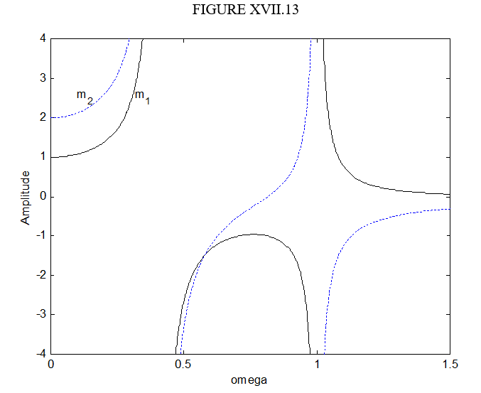
Where the amplitude is negative, the oscillations are out of phase with the force \( F\). The amplitudes go to infinity (remember we are assuming here zero damping) at the two frequencies where the denominators of Equations \( \ref{17.12.10}\) and \( \ref{17.12.11}\) are zero. The amplitude of the motion of \( m_{2}\) is zero when the numerator of Equation \( \ref{17.12.11}\) is zero. This is at an angular frequency of \( \sqrt{\frac{(k_{1}+k_{2})}{m_{1}}}\), which is just the angular frequency of the motion of \( m_{1}\) held by the two springs between two fixed points. In our numerical example, this is \( \omega\ =\ \sqrt{\frac{2}{3}}\ =\ 0.8165\). This is an example of antiresonance.