
5.4: Self-oscillations and Phase Locking
- Page ID
- 34773

\( \newcommand{\vecs}[1]{\overset { \scriptstyle \rightharpoonup} {\mathbf{#1}} } \)
\( \newcommand{\vecd}[1]{\overset{-\!-\!\rightharpoonup}{\vphantom{a}\smash {#1}}} \)
\( \newcommand{\id}{\mathrm{id}}\) \( \newcommand{\Span}{\mathrm{span}}\)
( \newcommand{\kernel}{\mathrm{null}\,}\) \( \newcommand{\range}{\mathrm{range}\,}\)
\( \newcommand{\RealPart}{\mathrm{Re}}\) \( \newcommand{\ImaginaryPart}{\mathrm{Im}}\)
\( \newcommand{\Argument}{\mathrm{Arg}}\) \( \newcommand{\norm}[1]{\| #1 \|}\)
\( \newcommand{\inner}[2]{\langle #1, #2 \rangle}\)
\( \newcommand{\Span}{\mathrm{span}}\)
\( \newcommand{\id}{\mathrm{id}}\)
\( \newcommand{\Span}{\mathrm{span}}\)
\( \newcommand{\kernel}{\mathrm{null}\,}\)
\( \newcommand{\range}{\mathrm{range}\,}\)
\( \newcommand{\RealPart}{\mathrm{Re}}\)
\( \newcommand{\ImaginaryPart}{\mathrm{Im}}\)
\( \newcommand{\Argument}{\mathrm{Arg}}\)
\( \newcommand{\norm}[1]{\| #1 \|}\)
\( \newcommand{\inner}[2]{\langle #1, #2 \rangle}\)
\( \newcommand{\Span}{\mathrm{span}}\) \( \newcommand{\AA}{\unicode[.8,0]{x212B}}\)
\( \newcommand{\vectorA}[1]{\vec{#1}} % arrow\)
\( \newcommand{\vectorAt}[1]{\vec{\text{#1}}} % arrow\)
\( \newcommand{\vectorB}[1]{\overset { \scriptstyle \rightharpoonup} {\mathbf{#1}} } \)
\( \newcommand{\vectorC}[1]{\textbf{#1}} \)
\( \newcommand{\vectorD}[1]{\overrightarrow{#1}} \)
\( \newcommand{\vectorDt}[1]{\overrightarrow{\text{#1}}} \)
\( \newcommand{\vectE}[1]{\overset{-\!-\!\rightharpoonup}{\vphantom{a}\smash{\mathbf {#1}}}} \)
\( \newcommand{\vecs}[1]{\overset { \scriptstyle \rightharpoonup} {\mathbf{#1}} } \)
\( \newcommand{\vecd}[1]{\overset{-\!-\!\rightharpoonup}{\vphantom{a}\smash {#1}}} \)
\(\newcommand{\avec}{\mathbf a}\) \(\newcommand{\bvec}{\mathbf b}\) \(\newcommand{\cvec}{\mathbf c}\) \(\newcommand{\dvec}{\mathbf d}\) \(\newcommand{\dtil}{\widetilde{\mathbf d}}\) \(\newcommand{\evec}{\mathbf e}\) \(\newcommand{\fvec}{\mathbf f}\) \(\newcommand{\nvec}{\mathbf n}\) \(\newcommand{\pvec}{\mathbf p}\) \(\newcommand{\qvec}{\mathbf q}\) \(\newcommand{\svec}{\mathbf s}\) \(\newcommand{\tvec}{\mathbf t}\) \(\newcommand{\uvec}{\mathbf u}\) \(\newcommand{\vvec}{\mathbf v}\) \(\newcommand{\wvec}{\mathbf w}\) \(\newcommand{\xvec}{\mathbf x}\) \(\newcommand{\yvec}{\mathbf y}\) \(\newcommand{\zvec}{\mathbf z}\) \(\newcommand{\rvec}{\mathbf r}\) \(\newcommand{\mvec}{\mathbf m}\) \(\newcommand{\zerovec}{\mathbf 0}\) \(\newcommand{\onevec}{\mathbf 1}\) \(\newcommand{\real}{\mathbb R}\) \(\newcommand{\twovec}[2]{\left[\begin{array}{r}#1 \\ #2 \end{array}\right]}\) \(\newcommand{\ctwovec}[2]{\left[\begin{array}{c}#1 \\ #2 \end{array}\right]}\) \(\newcommand{\threevec}[3]{\left[\begin{array}{r}#1 \\ #2 \\ #3 \end{array}\right]}\) \(\newcommand{\cthreevec}[3]{\left[\begin{array}{c}#1 \\ #2 \\ #3 \end{array}\right]}\) \(\newcommand{\fourvec}[4]{\left[\begin{array}{r}#1 \\ #2 \\ #3 \\ #4 \end{array}\right]}\) \(\newcommand{\cfourvec}[4]{\left[\begin{array}{c}#1 \\ #2 \\ #3 \\ #4 \end{array}\right]}\) \(\newcommand{\fivevec}[5]{\left[\begin{array}{r}#1 \\ #2 \\ #3 \\ #4 \\ #5 \\ \end{array}\right]}\) \(\newcommand{\cfivevec}[5]{\left[\begin{array}{c}#1 \\ #2 \\ #3 \\ #4 \\ #5 \\ \end{array}\right]}\) \(\newcommand{\mattwo}[4]{\left[\begin{array}{rr}#1 \amp #2 \\ #3 \amp #4 \\ \end{array}\right]}\) \(\newcommand{\laspan}[1]{\text{Span}\{#1\}}\) \(\newcommand{\bcal}{\cal B}\) \(\newcommand{\ccal}{\cal C}\) \(\newcommand{\scal}{\cal S}\) \(\newcommand{\wcal}{\cal W}\) \(\newcommand{\ecal}{\cal E}\) \(\newcommand{\coords}[2]{\left\{#1\right\}_{#2}}\) \(\newcommand{\gray}[1]{\color{gray}{#1}}\) \(\newcommand{\lgray}[1]{\color{lightgray}{#1}}\) \(\newcommand{\rank}{\operatorname{rank}}\) \(\newcommand{\row}{\text{Row}}\) \(\newcommand{\col}{\text{Col}}\) \(\renewcommand{\row}{\text{Row}}\) \(\newcommand{\nul}{\text{Nul}}\) \(\newcommand{\var}{\text{Var}}\) \(\newcommand{\corr}{\text{corr}}\) \(\newcommand{\len}[1]{\left|#1\right|}\) \(\newcommand{\bbar}{\overline{\bvec}}\) \(\newcommand{\bhat}{\widehat{\bvec}}\) \(\newcommand{\bperp}{\bvec^\perp}\) \(\newcommand{\xhat}{\widehat{\xvec}}\) \(\newcommand{\vhat}{\widehat{\vvec}}\) \(\newcommand{\uhat}{\widehat{\uvec}}\) \(\newcommand{\what}{\widehat{\wvec}}\) \(\newcommand{\Sighat}{\widehat{\Sigma}}\) \(\newcommand{\lt}{<}\) \(\newcommand{\gt}{>}\) \(\newcommand{\amp}{&}\) \(\definecolor{fillinmathshade}{gray}{0.9}\)The motivation for B. van der Pol to develop his method was the analysis of one more type of oscillatory motion: self-oscillations. Several systems, e.g., electronic rf amplifiers with positive feedback, and optical media with quantum level population inversion, provide convenient means for the compensation, and even over-compensation of the intrinsic energy losses in oscillators. Phenomenologically, this effect may be described as the change of sign of the damping coefficient \(\delta\) from positive to negative. Since for small oscillations the equation of motion is still linear, we may use Eq. (9) to describe its general solution. This equation shows that at \(\delta<0\), even infinitesimal deviations from equilibrium (say, due to unavoidable fluctuations) lead to oscillations with exponentially growing amplitude. Of course, in any real system such growth cannot persist infinitely, and shall be limited by this or that effect - e.g., in the above examples, respectively, by amplifier’s saturation and quantum level population’s exhaustion.
In many cases, the amplitude limitation may be described reasonably well by making the following replacement: \[2 \delta \ddot{q} \rightarrow 2 \delta \dot{q}+\beta \dot{q}^{3},\] with \(\beta>0\). Let us analyze the effects of such nonlinear damping, applying the van der Pol’s approach to the corresponding homogeneous differential equation (which is also known under his name): \[\ddot{q}+2 \delta \ddot{q}+\beta \dot{q}^{3}+\omega_{0}^{2} q=0 \text {. }\] Carrying out the dissipative and detuning terms to the right-hand side, and taking them for \(f\) in the canonical Eq. (38), we can easily calculate the right-hand sides of the reduced equations (57a), getting 22 \[\begin{gathered} \dot{A}=-\delta(A) A, \quad \text { where } \delta(A) \equiv \delta+\frac{3}{8} \beta \omega^{2} A^{2}, \\ A \dot{\varphi}=\xi A . \end{gathered}\] The last of these equations has exactly the same form as Eq. (58b) for the case of decaying oscillations and hence shows that the self-oscillations (if they happen, i.e. if \(A \neq 0\) ) have the own frequency \(\omega_{0}\) of the oscillator - cf. Eq. (59). However, Eq. (63a) is more substantive. If the initial damping \(\delta\) is positive, it has only the trivial fixed point, \(A_{0}=0\) (that describes the oscillator at rest), but if \(\delta\) is negative, there is also another fixed point,
\[A_{1}=\left(\frac{8|\delta|}{3 \beta \omega^{2}}\right)^{1 / 2}, \quad \text { for } \delta<0\] which describes steady self-oscillations with a non-zero amplitude \(A_{1}\).
Let us apply the general approach discussed in Sec. 3.2, the linearization of equations of motion, to this reduced equation. For the trivial fixed point \(A_{0}=0\), the linearization of Eq. (63a) is reduced to discarding the nonlinear term in the definition of the amplitude-dependent damping \(\delta(A)\). The resulting linear equation evidently shows that the system’s equilibrium point, \(A=A_{0}=0\), is stable at \(\delta>0\) and unstable at \(\delta<0\). (We have already discussed this self-excitation condition above.) On the other hand, the linearization of near the non-trivial fixed point \(A_{1}\) requires a bit more math: in the first order in \(\widetilde{A} \equiv A-A_{1} \rightarrow 0\), we get \[\dot{\widetilde{A}} \equiv \dot{A}=-\delta\left(A_{1}+\widetilde{A}\right)-\frac{3}{8} \beta \omega^{2}\left(A_{1}+\widetilde{A}\right)^{3} \approx-\delta \widetilde{A}-\frac{3}{8} \beta \omega^{2} 3 A_{1}^{2} \widetilde{A}=(-\delta+3 \delta) \widetilde{A}=2 \delta \widetilde{A},\] where Eq. (64) has been used to eliminate \(A_{1}\). We see that the fixed point \(A_{1}\) (and hence the whole process) is stable as soon as it exists \((\delta<0)-\) similarly to the situation in our "testbed problem" (Figure 2.1), besides that in our current, dissipative system, the stability is "actual" rather than "orbital" - see Sec. 6 for more on this issue.
Now let us consider another important problem: the effect of an external sinusoidal force on a self-excited oscillator. If the force is sufficiently small, its effects on the self-excitation condition and the oscillation amplitude are negligible. However, if the frequency \(\omega\) of such a weak force is close to the own frequency \(\omega_{0}\) of the oscillator, it may lead to a very important effect of phase locking \(^{23}\) - also called the "synchronization", though the latter term also has a much broader meaning. At this effect, the oscillation frequency deviates from \(\omega_{0}\), and becomes exactly equal to the external force’s frequency \(\omega\), within a certain range \[-\Delta \leq \omega-\omega_{0}<+\Delta .\] To prove this fact, and also to calculate the phase-locking range width \(2 \Delta\), we may repeat the calculation of the right-hand sides of the reduced equations (57a), adding the term \(f_{0} \cos \omega t\) to the righthand side of Eq. (62) - cf. Eqs. (42)-(43). This addition modifies Eqs. (63) as follows: 24 \[\begin{aligned} &\dot{A}=-\delta(A) A+\frac{f_{0}}{2 \omega} \sin \varphi, \\ &A \dot{\varphi}=\xi A+\frac{f_{0}}{2 \omega} \cos \varphi . \end{aligned}\] If the system is self-excited, and the external force is weak, its effect on the oscillation amplitude is small, and in the first approximation in \(f_{0}\) we can take \(A\) to be constant and equal to the value \(A_{1}\) given by Eq. (64). Plugging this approximation into Eq. (67b), we get a very simple equation \({ }^{25}\)
\[\ \text{Phase locking equation}\quad\quad\quad\quad\dot{\varphi}=\xi+\Delta \cos \varphi\]
where in our current case \[\Delta \equiv \frac{f_{0}}{2 \omega A_{1}} .\] Within the range \(-|\Delta|<\xi<+|\Delta|\), Eq. (68) has two fixed points on each \(2 \pi\)-segment of the variable \(\varphi\) : \[\varphi_{\pm}=\pm \cos ^{-1}\left(-\frac{\xi}{\Delta}\right)+2 \pi n .\] It is easy to linearize Eq. (68) near each point to analyze their stability in our usual way; however, let me use this case to demonstrate another convenient way to do this in 1D systems, using the so-called phase plane - the plot of the right-hand side of Eq. (68) as a function of \(\varphi\) - see Figure 5 .
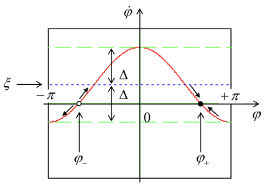
Figure 5.5. The phase plane of a phaselocked oscillator, for the particular case \(\xi=\Delta / 2, f_{0}>0\).
Since according to Eq. (68), positive values of this function correspond to the growth of \(\varphi\) in time and vice versa, we may draw the arrows showing the direction of phase evolution. From this graphics, it is clear that one of these fixed points (for \(f_{0}>0, \varphi_{+}\)) is stable, while its counterpart (in this case, \(\varphi\).) is unstable. Hence the magnitude of \(\Delta\) given by Eq. (69) is indeed the phase-locking range (or rather it half) that we wanted to find. Note that the range is proportional to the amplitude of the phaselocking signal - perhaps the most important feature of this effect.
To complete our simple analysis, based on the assumption of fixed oscillation amplitude, we need to find the condition of its validity. For that, we may linearize Eq. (67a), for the stationary case, near the value \(A_{1}\), just as we have done in Eq. (65) for the transient process. The stationary result, \[\widetilde{A} \equiv A-A_{1}=\frac{1}{2|\delta|} \frac{f_{0}}{2 \omega} \sin \varphi_{\pm} \approx A_{1}\left|\frac{\Delta}{2 \delta}\right| \sin \varphi_{\pm},\] shows that our assumption, \(|\widetilde{A}|<<A_{1}\), and hence the final result (69), are valid if the calculated phaselocking range \(2 \Delta\) is much smaller than \(4|\delta|\).
\({ }^{22}\) For that, one needs to use the trigonometric identity \(\sin ^{3} \Psi=(3 / 4) \sin \Psi-(1 / 4) \sin 3 \Psi-\) see, e.g., MA Eq. (3.4).
\({ }^{23}\) Apparently, the mutual phase locking of two pendulum clocks was first noticed by the same \(C\). Huygens.
\({ }^{24}\) Actually, this result should be evident, even without calculations, from the comparison of Eqs. (60) and (63).
\({ }_{25}\) This equation is ubiquitous in phase-locking systems, including even some digital electronic circuits used for that purpose - at the proper re-definition of the phase difference \(\varphi\).