5.5: Parametric Excitation

In both problems solved in the last section, the stability analysis was easy because it could be carried out for just one slow variable, either amplitude or phase. More generally, such an analysis of the reduced equations involves both these variables. A classical example of such a situation is provided by one important physical phenomenon - the parametric excitation of oscillations. A simple example of such excitation is given by a pendulum with a variable parameter, for example, the suspension length \(l(t)\) - see Figure 6. Experiments (including those with playground swings :-) and numerical simulations show that if the length is changed (modulated) periodically, with some frequency \(2 \omega\) that is close to \(2 \omega_{0}\), and a sufficiently large swing \(\Delta l\), the equilibrium position of the pendulum becomes unstable, and it starts oscillating with frequency \(\omega\) equal exactly to the half of the modulation frequency (and hence only approximately equal to the average frequency \(\omega_{0}\) of the oscillator).

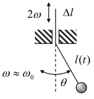Figure 5.6. Parametric excitation of a pendulum.

For an elementary analysis of this effect, we may consider the simplest case when the oscillations are small. At the lowest point \((\theta=0)\), where the pendulum moves with the highest velocity \(v_{\text {max }}\), the suspension string’s tension \(\mathscr{T}\) is higher than \(m g\) by the centripetal force: \(\mathscr{T}_{\max }=m g+m v_{\max }^{2} / l\). On the contrary, at the maximum deviation of the pendulum from the equilibrium, the force is lower than \(m g\), because of the string’s tilt: \(\mathscr{T}_{\min }=m g \cos \theta_{\max }\). Using the energy conservation, \(E=m v_{\max }^{2} / 2=\) \(m g l\left(1-\cos \theta_{\max }\right)\), we may express these values as \(\mathscr{T}_{\max }=m g+2 E / l\) and \(\mathscr{T}_{\min }=m g-E / l\). Now, if during each oscillation period the string is pulled up slightly by \(\Delta l\) (with \(|\Delta l|<<l\) ) at each of its two passages through the lowest point, and is let to go down by the same amount at each of two points of the maximum deviation, the net work of the external force per period is positive: \[\mathscr{W} \approx 2\left(\mathscr{T}_{\max }-\mathscr{T}_{\min }\right) \Delta l \approx 6 \frac{\Delta l}{l} E,\] and hence increases the oscillator’s energy. If the parameter swing \(\Delta l\) is sufficient, this increase may overcompensate the energy drained out by damping during the same period. Quantitatively, Eq. (10) shows that low damping \(\left(\delta<\omega_{0}\right)\) leads to the following energy decrease, \[\Delta E \approx-4 \pi \frac{\delta}{\omega_{0}} E \text {, }\] per oscillation period. Comparing Eqs. (72) and (73), we see that the net energy flow into the oscillations is positive, \(\mathscr{W}+\Delta E>0\), i.e. oscillation amplitude has to grow if \(^{26}\) \[\frac{\Delta l}{l}>\frac{2 \pi \delta}{3 \omega_{0}} \equiv \frac{\pi}{3 Q} .\] Since this result is independent of the oscillation energy \(E\), the growth of energy and amplitude is exponential (until \(E\) becomes so large that some of our assumptions fail), so that Eq. (74) is the condition of parametric excitation - in this simple model.

However, this result does not account for a possible difference between the oscillation frequency \(\omega\) and the eigenfrequency \(\omega_{0}\), and also does not clarify whether the best phase shift between the oscillations and parameter modulation, assumed in the above calculation, may be sustained automatically. To address these issues, we may apply the van der Pol approach to a simple but reasonable model: \[\ddot{q}+2 \delta \ddot{q}+\omega_{0}^{2}(1+\mu \cos 2 \omega t) q=0,\] describing the parametric excitation in a linear oscillator with a sinusoidal modulation of the parameter \(\omega_{0}^{2}(t)\). Rewriting this equation in the canonical form (38), \[\ddot{q}+\omega^{2} q=f(t, q, \dot{q}) \equiv-2 \delta \ddot{q}+2 \xi \omega q-\mu \omega_{0}^{2} q \cos 2 \omega t \text {, }\] and assuming that the dimensionless ratios \(\delta / \omega\) and \(|\xi| / \omega\), and the modulation depth \(\mu\) are all much less than 1, we may use general Eqs. (57a) to get the following reduced equations: \[\begin{aligned} &\dot{A}=-\delta A-\frac{\mu \omega}{4} A \sin 2 \varphi, \\ &A \dot{\varphi}=A \xi-\frac{\mu \omega}{4} A \cos 2 \varphi . \end{aligned}\] These equations evidently have a fixed point, with \(A_{0}=0\), but its stability analysis (though possible) is not absolutely straightforward, because the phase \(\varphi\) of oscillations is undetermined at that point. In order to avoid this (technical rather than conceptual) difficulty, we may use, instead of the real amplitude and phase of oscillations, either their complex amplitude \(a=A \exp \{i \varphi\}\), or its Cartesian components \(u\) and \(v\)-see Eqs. (4). Indeed, for our function \(f\), Eq. (57b) gives \[\dot{a}=(-\delta+i \xi) a-i \frac{\mu \omega}{4} a^{*},\] while Eqs. (57c) yield \[\begin{aligned} &\dot{u}=-\delta u-\xi v-\frac{\mu \omega}{4} v, \\ &\dot{v}=-\delta v+\xi u-\frac{\mu \omega}{4} u . \end{aligned}\] We see that in contrast to Eqs. (77), in the Cartesian coordinates \(\{u, v\}\) the trivial fixed point \(a_{0}\) \(=0\) (i.e. \(\left.u_{0}=v_{0}=0\right)\) is absolutely regular. Moreover, equations (78)-(79) are already linear, so they do not require any additional linearization. Thus we may use the same approach as was already used in Secs. \(3.2\) and 5.1, i.e. look for the solution of Eqs. (79) in the exponential form \(\exp \{\lambda t\}\). However, now we are dealing with two variables and should allow them to have, for each value of \(\lambda\), a certain ratio \(u / v\). For that, we may take the partial solution in the form \[u=c_{u} e^{\lambda t}, \quad v=c_{v} e^{\lambda t} .\] where the constants \(c_{u}\) and \(c_{v}\) are frequently called the distribution coefficients. Plugging this solution into Eqs. (79), we get from them the following system of two linear algebraic equations: \[\begin{aligned} &(-\delta-\lambda) c_{u}+\left(-\xi-\frac{\mu \omega}{4}\right) c_{v}=0, \\ &\left(+\xi-\frac{\mu \omega}{4}\right) c_{u}+(-\delta-\lambda) c_{v}=0 . \end{aligned}\] The characteristic equation of this system, i.e. the condition of compatibility of Eqs. (81), \[\left|\begin{array}{cc} -\delta-\lambda & -\xi-\frac{\mu \omega}{4} \\ \xi-\frac{\mu \omega}{4} & -\delta-\lambda \end{array}\right| \equiv \lambda^{2}+2 \delta \lambda+\delta^{2}+\xi^{2}-\left(\frac{\mu \omega}{4}\right)^{2}=0\] has two roots: \[\lambda_{\pm}=-\delta \pm\left[\left(\frac{\mu \omega}{4}\right)^{2}-\xi^{2}\right]^{1 / 2}\] Requiring the fixed point to be unstable, \(\operatorname{Re} \lambda_{+}>0\), we get the parametric excitation condition \[\frac{\mu \omega}{4}>\left(\delta^{2}+\xi^{2}\right)^{1 / 2} .\] Thus the parametric excitation may indeed happen without any external phase control: the arising oscillations self-adjust their phase to pick up energy from the external source responsible for the periodic parameter variation.

Our key result (84) may be compared with two other calculations. First, in the case of negligible damping \((\delta=0)\), Eq. (84) turns into the condition \(\mu \omega / 4>|\xi|\). This result may be compared with the well-developed theory of the so-called Mathieu equation, whose canonical form is \[\frac{d^{2} y}{d v^{2}}+(a-2 b \cos 2 v) y=0 .\] With the substitutions \(y \rightarrow q, v \rightarrow \omega t, a \rightarrow\left(\omega_{0} / \omega\right)^{2}\), and \(b / a \rightarrow-\mu / 2\), this equation is just a particular case of Eq. (75) for \(\delta=0\). In terms of Eq. (85), our result (84) may be re-written just as \(b>|a-1|\), and is supposed to be valid for \(b<<1\). The boundaries given by this condition are shown with dashed lines in Figure 7 together with the numerically calculated \({ }^{27}\) stability boundaries for the Mathieu equation.

One can see that the van der Pol approximation works just fine within its applicability limit (and a bit beyond :-), though it fails to predict some other important features of the Mathieu equation, such as the existence of higher, more narrow regions of parametric excitation (at \(a \approx n^{2}\), i.e. \(\omega_{0} \approx \omega / n\), for all integer \(n\) ), and some spill-over of the stability region into the lower half-plane \(a<0 .{ }^{28}\) The reason for these failures is the fact that, as can be seen in Figure 7, these phenomena do not appear in the first approximation in the parameter modulation amplitude \(\mu \propto \varepsilon\), which is the realm of applicability of the reduced equations (79).

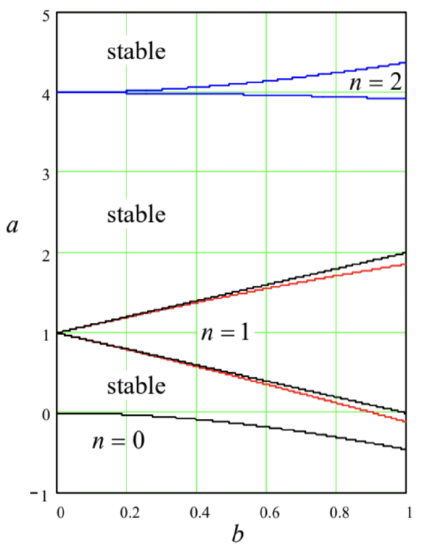
Figure 5.7. Stability boundaries of the Mathieu equation (85), as calculated: numerically (solid curves) and using the reduced equations (dashed straight lines). In the regions numbered by various \(n\), the trivial solution \(y=0\) of the equation is unstable, i.e. its general solution \(y(v)\) includes an exponentially growing term.

In the opposite case of non-zero damping but exact tuning \(\left(\xi=0, \omega \approx \omega_{0}\right)\), Eq. (84) becomes \[\mu>\frac{4 \delta}{\omega_{0}} \equiv \frac{2}{Q} \text {. }\] This condition may be compared with Eq. (74) by taking \(\Delta l / l=2 \mu\). The comparison shows that while the structure of these conditions is similar, the numerical coefficients are different by a factor close to 2 . The first reason for this difference is that the instant parameter change at optimal moments of time is more efficient than the smooth, sinusoidal variation described by (75). Even more significantly, the change of pendulum’s length modulates not only its frequency \(\omega_{0} \equiv(g / l)^{1 / 2}\) as Eq. (75) implies but also its mechanical impedance \(Z \equiv(g l)^{1 / 2}-\) the notion to be discussed in detail in the next chapter. (The analysis of the general case of the simultaneous modulation of \(\omega_{0}\) and \(Z\) is left for the reader’s exercise.)

Before moving on, let me summarize the most important differences between the parametric and forced oscillations:

(i) Parametric oscillations completely disappear outside of their excitation range, while the forced oscillations have a non-zero amplitude for any frequency and amplitude of the external force see Eq. (18).

(ii) Parametric excitation may be described by a linear homogeneous equation - e.g., Eq. (75) which cannot predict any finite oscillation amplitude within the excitation range, even at finite damping. In order to describe stationary parametric oscillations, some nonlinear effect has to be taken into account. (I am leaving analyses of such effects for the reader’s exercise - see Problems 13 and 14.)

One more important feature of the parametric oscillations will be discussed at the end of the next section.

---

\({ }^{26}\) A modulation of the pendulum’s mass (say, by periodic pumping water in and out of a suspended bottle) gives a qualitatively similar result. Note, however, that parametric oscillations cannot be excited by modulating any oscillator’s parameter - for example, oscillator’s damping coefficient (at least if it stays positive at all times), because its does not change the system’s energy, just the energy drain rate.

\({ }^{27}\) Such calculations are substantially simplified by the use of the so-called Floquet theorem, which is also the mathematical basis for the discussion of wave propagation in periodic media \(-\) see the next chapter.

\({ }^{28}\) This region (for \(b<1,-b^{2} / 2<a<0\) ) describes, in particular, the counter-intuitive stability of the so-called Kapitza pendulum - an inverted pendulum with the suspension point oscillated fast in the vertical direction - the effect first observed by Andrew Stephenson in 1908 .