5.9: Exercise Problems

5.1. For a system with the response function given by Eq. (17), prove Eq. (26) and use an approach different from the one used in Sec. 1, to derive Eq. (34).

Hint: You may like to use the Cauchy integral theorem and the Cauchy integral formula for analytical functions of a complex variable \({ }^{42}\)

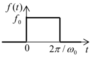
5.2. A square-wave pulse of force (see the figure on the right) is exerted on a linear oscillator with eigenfrequency \(\omega_{0}\) (with no damping), initially at rest. Calculate the law of motion \(q(t)\), sketch it, and interpret the result.

5.3. At \(t=0\), a sinusoidal external force \(F(t)=F_{0} \cos \omega t\), is exerted on a linear oscillator with eigenfrequency \(\omega_{0}\) and damping \(\delta\), which was at rest at \(t \leq 0\).

(i) Derive the general expression for the time evolution of the oscillator’s coordinate, and interpret the result.

(ii) Spell out the result for the exact resonance \(\left(\omega=\omega_{0}\right)\) in a system with low damping \(\left(\delta<<\omega_{0}\right)\), and, in particular, explore the limit \(\delta \rightarrow 0\).

5.4. A pulse of external force \(F(t)\), with a finite duration \(\tau\), is exerted on a linear oscillator, initially at rest in its equilibrium position. Neglecting dissipation, calculate the change of oscillator’s energy, using two different approaches, and compare the results.

5.5. For a system with the following Lagrangian function: \[L=\frac{m}{2} \dot{q}^{2}-\frac{\kappa}{2} q^{2}+\frac{\varepsilon}{2} \dot{q}^{2} q^{2},\] calculate the frequency of free oscillations as a function of their amplitude \(A\), at \(A \rightarrow 0\), using two different approaches.

5.6. For a system with the Lagrangian function \[L=\frac{m}{2} \dot{q}^{2}-\frac{\kappa}{2} q^{2}+\varepsilon \dot{q}^{4},\] with small parameter \(\varepsilon\), use the van der Pol method to find the frequency of free oscillations as a function of their amplitude.

5.7. On the plane \(\left[a_{1}, a_{2}\right]\) of two real, time-independent parameters \(a_{1}\) and \(a_{2}\), find the regions in which the fixed point of the following system of equations, \[\begin{aligned} &\dot{q}_{1}=a_{1}\left(q_{2}-q_{1}\right), \\ &\dot{q}_{2}=a_{2} q_{1}-q_{2}, \end{aligned}\] is unstable, and sketch the regions of each fixed point type \(-\) stable and unstable nodes, focuses, etc.

5.8. Solve Problem 3(ii) using the reduced equations (57), and compare the result with the exact solution.

5.9. Use the reduced equations to analyze forced oscillations in an oscillator with weak nonlinear damping, described by the following equation: \[\ddot{q}+2 \delta \dot{q}+\omega_{0}^{2} q+\beta \dot{q}^{3}=f_{0} \cos \omega t,\] with \(\omega \approx \omega_{0} ; \beta, \delta>0\); and \(\beta \omega A^{2}<<1\). In particular, find the stationary amplitude of the forced oscillations and analyze their stability. Discuss the effect(s) of the nonlinear term on the resonance.

5.10. Within the approach discussed in Sec. 4, calculate the average frequency of a self-oscillator outside of the range of its phase-locking by an external sinusoidal force.

5.11.* Use the reduced equations to analyze the stability of the forced nonlinear oscillations described by the Duffing equation (43). Relate the result to the slope of resonance curves (Figure 4).

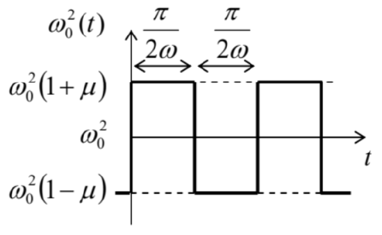
5.12. Use the van der Pol method to find the condition of parametric excitation of the oscillator described by the following equation: \[\ddot{q}+2 \delta \dot{q}+\omega_{0}^{2}(t) q=0,\] where \(\omega_{0}^{2}(t)\) is the square-wave function shown in the figure on the right, with \(\omega \approx \omega_{0}\).

5.13. Use the van der Pol method to analyze parametric excitation of an oscillator with weak nonlinear damping, described by the following equation: \[\ddot{q}+2 \delta \ddot{q}+\beta \dot{q}^{3}+\omega_{0}{ }^{2}(1+\mu \cos 2 \omega t) q=0 \text {, }\] with \(\omega \approx \omega_{0} ; \beta, \delta>0 ;\) and \(\mu, \beta \omega A^{2}<<1\). In particular, find the amplitude of stationary oscillations and analyze their stability.

5.14. \({ }^{*}\) Adding nonlinear term \(\alpha q^{3}\) to the left-hand side of Eq. (75),

(i) find the corresponding addition to the reduced equations,

(ii) calculate the stationary amplitude \(A\) of the parametric oscillations,

(iii) find the type and stability of each fixed point of the reduced equations,

(iv) sketch the Poincare phase planes of the system in major parameter regions.

5.15. Use the van der Pol method to find the condition of parametric excitation of an oscillator with weak modulation of both the effective mass \(m(t)=m_{0}\left(1+\mu_{m} \cos 2 \omega t\right)\) and the effective spring constant \(\kappa(t)=\kappa_{0}\left[1+\mu_{\kappa} \cos (2 \omega t-\psi)\right]\), with the same frequency \(2 \omega \approx 2 \omega_{0}\), at arbitrary modulation depths ratio \(\mu_{m} / \mu_{k}\) and phase shift \(\psi\). Interpret the result in terms of modulation of the instantaneous frequency \(\omega(t) \equiv[\kappa(t) / m(t)]^{1 / 2}\) and the mechanical impedance \(Z(t) \equiv[\kappa(t) m(t)]^{1 / 2}\) of the oscillator.

5.16. \({ }^{*}\) Find the condition of parametric excitation of a nonlinear oscillator described by the following equation: \[\ddot{q}+2 \delta \dot{q}+\omega_{0}^{2} q+\gamma q^{2}=f_{0} \cos 2 \omega t,\] with sufficiently small \(\delta, \gamma, f_{0}\), and \(\xi \equiv \omega-\omega_{0}\).

5.17. Find the condition of stability of the equilibrium point \(q=0\) of a parametric oscillator described by Eq. (75), in the limit when \(\delta<<\left|\omega_{0}\right|<<\omega\) and \(\mu<<1\). Use the result to analyze stability of the Kapitza pendulum mentioned in Sec. 5 .

---

\({ }^{42}\) See, e.g., MA Eq. (15.1).