
5.8: Harmonic and Subharmonic Oscillations
- Page ID
- 58631
\( \newcommand{\vecs}[1]{\overset { \scriptstyle \rightharpoonup} {\mathbf{#1}} } \)
\( \newcommand{\vecd}[1]{\overset{-\!-\!\rightharpoonup}{\vphantom{a}\smash {#1}}} \)
\( \newcommand{\id}{\mathrm{id}}\) \( \newcommand{\Span}{\mathrm{span}}\)
( \newcommand{\kernel}{\mathrm{null}\,}\) \( \newcommand{\range}{\mathrm{range}\,}\)
\( \newcommand{\RealPart}{\mathrm{Re}}\) \( \newcommand{\ImaginaryPart}{\mathrm{Im}}\)
\( \newcommand{\Argument}{\mathrm{Arg}}\) \( \newcommand{\norm}[1]{\| #1 \|}\)
\( \newcommand{\inner}[2]{\langle #1, #2 \rangle}\)
\( \newcommand{\Span}{\mathrm{span}}\)
\( \newcommand{\id}{\mathrm{id}}\)
\( \newcommand{\Span}{\mathrm{span}}\)
\( \newcommand{\kernel}{\mathrm{null}\,}\)
\( \newcommand{\range}{\mathrm{range}\,}\)
\( \newcommand{\RealPart}{\mathrm{Re}}\)
\( \newcommand{\ImaginaryPart}{\mathrm{Im}}\)
\( \newcommand{\Argument}{\mathrm{Arg}}\)
\( \newcommand{\norm}[1]{\| #1 \|}\)
\( \newcommand{\inner}[2]{\langle #1, #2 \rangle}\)
\( \newcommand{\Span}{\mathrm{span}}\) \( \newcommand{\AA}{\unicode[.8,0]{x212B}}\)
\( \newcommand{\vectorA}[1]{\vec{#1}} % arrow\)
\( \newcommand{\vectorAt}[1]{\vec{\text{#1}}} % arrow\)
\( \newcommand{\vectorB}[1]{\overset { \scriptstyle \rightharpoonup} {\mathbf{#1}} } \)
\( \newcommand{\vectorC}[1]{\textbf{#1}} \)
\( \newcommand{\vectorD}[1]{\overrightarrow{#1}} \)
\( \newcommand{\vectorDt}[1]{\overrightarrow{\text{#1}}} \)
\( \newcommand{\vectE}[1]{\overset{-\!-\!\rightharpoonup}{\vphantom{a}\smash{\mathbf {#1}}}} \)
\( \newcommand{\vecs}[1]{\overset { \scriptstyle \rightharpoonup} {\mathbf{#1}} } \)
\( \newcommand{\vecd}[1]{\overset{-\!-\!\rightharpoonup}{\vphantom{a}\smash {#1}}} \)
\(\newcommand{\avec}{\mathbf a}\) \(\newcommand{\bvec}{\mathbf b}\) \(\newcommand{\cvec}{\mathbf c}\) \(\newcommand{\dvec}{\mathbf d}\) \(\newcommand{\dtil}{\widetilde{\mathbf d}}\) \(\newcommand{\evec}{\mathbf e}\) \(\newcommand{\fvec}{\mathbf f}\) \(\newcommand{\nvec}{\mathbf n}\) \(\newcommand{\pvec}{\mathbf p}\) \(\newcommand{\qvec}{\mathbf q}\) \(\newcommand{\svec}{\mathbf s}\) \(\newcommand{\tvec}{\mathbf t}\) \(\newcommand{\uvec}{\mathbf u}\) \(\newcommand{\vvec}{\mathbf v}\) \(\newcommand{\wvec}{\mathbf w}\) \(\newcommand{\xvec}{\mathbf x}\) \(\newcommand{\yvec}{\mathbf y}\) \(\newcommand{\zvec}{\mathbf z}\) \(\newcommand{\rvec}{\mathbf r}\) \(\newcommand{\mvec}{\mathbf m}\) \(\newcommand{\zerovec}{\mathbf 0}\) \(\newcommand{\onevec}{\mathbf 1}\) \(\newcommand{\real}{\mathbb R}\) \(\newcommand{\twovec}[2]{\left[\begin{array}{r}#1 \\ #2 \end{array}\right]}\) \(\newcommand{\ctwovec}[2]{\left[\begin{array}{c}#1 \\ #2 \end{array}\right]}\) \(\newcommand{\threevec}[3]{\left[\begin{array}{r}#1 \\ #2 \\ #3 \end{array}\right]}\) \(\newcommand{\cthreevec}[3]{\left[\begin{array}{c}#1 \\ #2 \\ #3 \end{array}\right]}\) \(\newcommand{\fourvec}[4]{\left[\begin{array}{r}#1 \\ #2 \\ #3 \\ #4 \end{array}\right]}\) \(\newcommand{\cfourvec}[4]{\left[\begin{array}{c}#1 \\ #2 \\ #3 \\ #4 \end{array}\right]}\) \(\newcommand{\fivevec}[5]{\left[\begin{array}{r}#1 \\ #2 \\ #3 \\ #4 \\ #5 \\ \end{array}\right]}\) \(\newcommand{\cfivevec}[5]{\left[\begin{array}{c}#1 \\ #2 \\ #3 \\ #4 \\ #5 \\ \end{array}\right]}\) \(\newcommand{\mattwo}[4]{\left[\begin{array}{rr}#1 \amp #2 \\ #3 \amp #4 \\ \end{array}\right]}\) \(\newcommand{\laspan}[1]{\text{Span}\{#1\}}\) \(\newcommand{\bcal}{\cal B}\) \(\newcommand{\ccal}{\cal C}\) \(\newcommand{\scal}{\cal S}\) \(\newcommand{\wcal}{\cal W}\) \(\newcommand{\ecal}{\cal E}\) \(\newcommand{\coords}[2]{\left\{#1\right\}_{#2}}\) \(\newcommand{\gray}[1]{\color{gray}{#1}}\) \(\newcommand{\lgray}[1]{\color{lightgray}{#1}}\) \(\newcommand{\rank}{\operatorname{rank}}\) \(\newcommand{\row}{\text{Row}}\) \(\newcommand{\col}{\text{Col}}\) \(\renewcommand{\row}{\text{Row}}\) \(\newcommand{\nul}{\text{Nul}}\) \(\newcommand{\var}{\text{Var}}\) \(\newcommand{\corr}{\text{corr}}\) \(\newcommand{\len}[1]{\left|#1\right|}\) \(\newcommand{\bbar}{\overline{\bvec}}\) \(\newcommand{\bhat}{\widehat{\bvec}}\) \(\newcommand{\bperp}{\bvec^\perp}\) \(\newcommand{\xhat}{\widehat{\xvec}}\) \(\newcommand{\vhat}{\widehat{\vvec}}\) \(\newcommand{\uhat}{\widehat{\uvec}}\) \(\newcommand{\what}{\widehat{\wvec}}\) \(\newcommand{\Sighat}{\widehat{\Sigma}}\) \(\newcommand{\lt}{<}\) \(\newcommand{\gt}{>}\) \(\newcommand{\amp}{&}\) \(\definecolor{fillinmathshade}{gray}{0.9}\)Figure 13 shows the numerically calculated \({ }^{37}\) transient process and stationary oscillations in a linear oscillator and a very representative nonlinear system, the pendulum described by Eq. (42), both with the same \(\omega_{0}\). Both systems are driven by a sinusoidal external force of the same amplitude and frequency - in this illustration, equal to the small-oscillation own frequency \(\omega_{0}\) of both systems. The plots show that despite a very substantial amplitude of the pendulum oscillations (the angle amplitude of about one radian), their waveform remains almost exactly sinusoidal. \({ }^{38}\) On the other hand, the nonlinearity affects the oscillation amplitude very substantially. These results imply that the corresponding reduced equations (60), which are based on the assumption (41), may work very well far beyond its formal restriction \(|q|<<1\).
Still, the waveform of oscillations in a nonlinear system always differs from that of the applied force \(-\) in our case, from the sine function of frequency \(\omega\). This fact is frequently formulated as the generation, by the system, of higher harmonics. Indeed, the Fourier theorem tells us that any nonsinusoidal periodic function of time may be represented as a sum of its basic harmonic of frequency \(\omega\) and higher harmonics with frequencies \(n \omega\), with integer \(n>1\).
Note that an effective generation of higher harmonics is only possible with adequate nonlinearity of the system. For example, consider the nonlinear term \(\alpha q^{3}\) used in the equations explored in Secs. 2 and 3. If the waveform \(q(t)\) is sinusoidal, such term will have only the basic \(\left(1^{\text {st }}\right)\) and the \(3^{\text {rd }}\) harmonics see, e.g., Eq. (50). As another example, the "pendulum nonlinearity" \(\sin q\) cannot produce, without a time-independent component ("bias") in \(q(t)\), any even harmonic, including the \(2^{\text {nd }}\) one. The most efficient generation of harmonics may be achieved using systems with the sharpest nonlinearities - e.g., semiconductor diodes whose current may follow an exponential dependence on the applied voltage through several orders of magnitude. \({ }^{39}\)
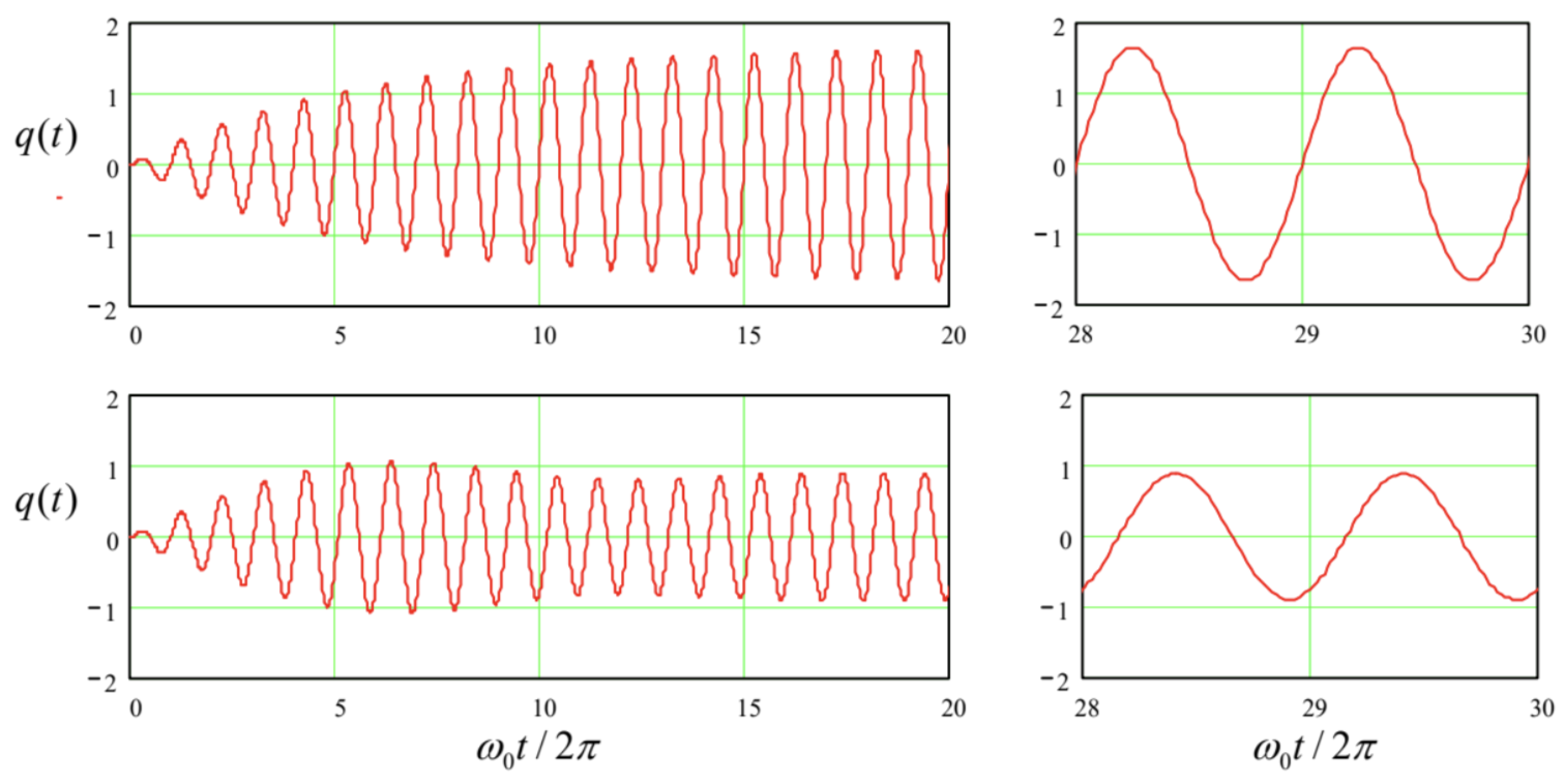
Figure 5.13. The oscillations induced by a similar sinusoidal external force (turned on at \(t=0\) ) in two systems with the same small-oscillation frequency \(\omega_{0}\) and low damping: a linear oscillator (two top panels) and a pendulum (two bottom panels). In all cases, \(\delta / \omega_{0}=0.03, f_{0}=0.1\), and \(\omega=\omega_{0}\).
Another way to increase the contents of an \(n^{\text {th }}\) higher harmonic in a nonlinear oscillator is to reduce the excitation frequency \(\omega\) to \(\sim \omega_{0} / n\), so that the oscillator resonated at the frequency \(n \omega \approx \omega_{0}\) of the desired harmonic. For example, Figure 14a shows the oscillations in a pendulum described by the same Eq. (42), but driven at frequency \(\omega=\omega_{0} / 3\). One can see that the \(3^{\text {rd }}\) harmonic amplitude may be comparable with that of the basic harmonic, especially if the external frequency is additionally lowered (Figure 14b) to accommodate for the deviation of the effective frequency \(\omega_{0}(A)\) of own oscillations from its small-oscillation value \(\omega_{0}-\) see Eq. (49), Figure 4, and their discussion in Sec. 2 above.
However, numerical modeling of nonlinear oscillators, as well as experiments with their physical implementations, bring more surprises. For example, the bottom panel of Figure 15 shows oscillations in a pendulum under the effect of a strong sinusoidal force with a frequency \(\omega\) close to \(3 \omega_{0}\). One can see that at some parameter values and initial conditions, the system’s oscillation spectrum is heavily contributed (almost dominated) by the \(3^{\text {rd }}\) subharmonic, i.e. the Fourier component of frequency \(\omega / 3 \approx \omega_{0}\).
This counter-intuitive phenomenon of such subharmonic generation may be explained as follows. Let us assume that subharmonic oscillations of frequency \(\omega / 3 \approx \omega_{0}\) have somehow appeared, and coexist with the forced oscillations of frequency \(3 \omega\):
\[q(t) \approx A \cos \Psi+A_{\text {sub }} \cos \Psi_{\text {sub }}, \quad \text { where } \Psi \equiv \omega t-\varphi, \quad \Psi_{\text {sub }} \equiv \frac{\omega t}{3}-\varphi_{\text {sub }} .\] Then the leading nonlinear term, \(\alpha q^{3}\), of the Taylor expansion of the pendulum’s nonlinearity \(\sin q\), is proportional to \[\begin{aligned} q^{3} &=\left(A \cos \Psi+A_{\text {sub }} \cos \Psi_{\text {sub }}\right)^{3} \\ & \equiv A^{3} \cos ^{3} \Psi+3 A^{2} A_{\text {sub }} \cos ^{2} \Psi \cos \Psi_{\text {sub }}+3 A A_{\text {sub }}^{2} \cos \Psi \cos ^{2} \Psi_{\text {sub }}+A_{\text {sub }}^{3} \cos ^{3} \Psi_{\text {sub }} \end{aligned}\]
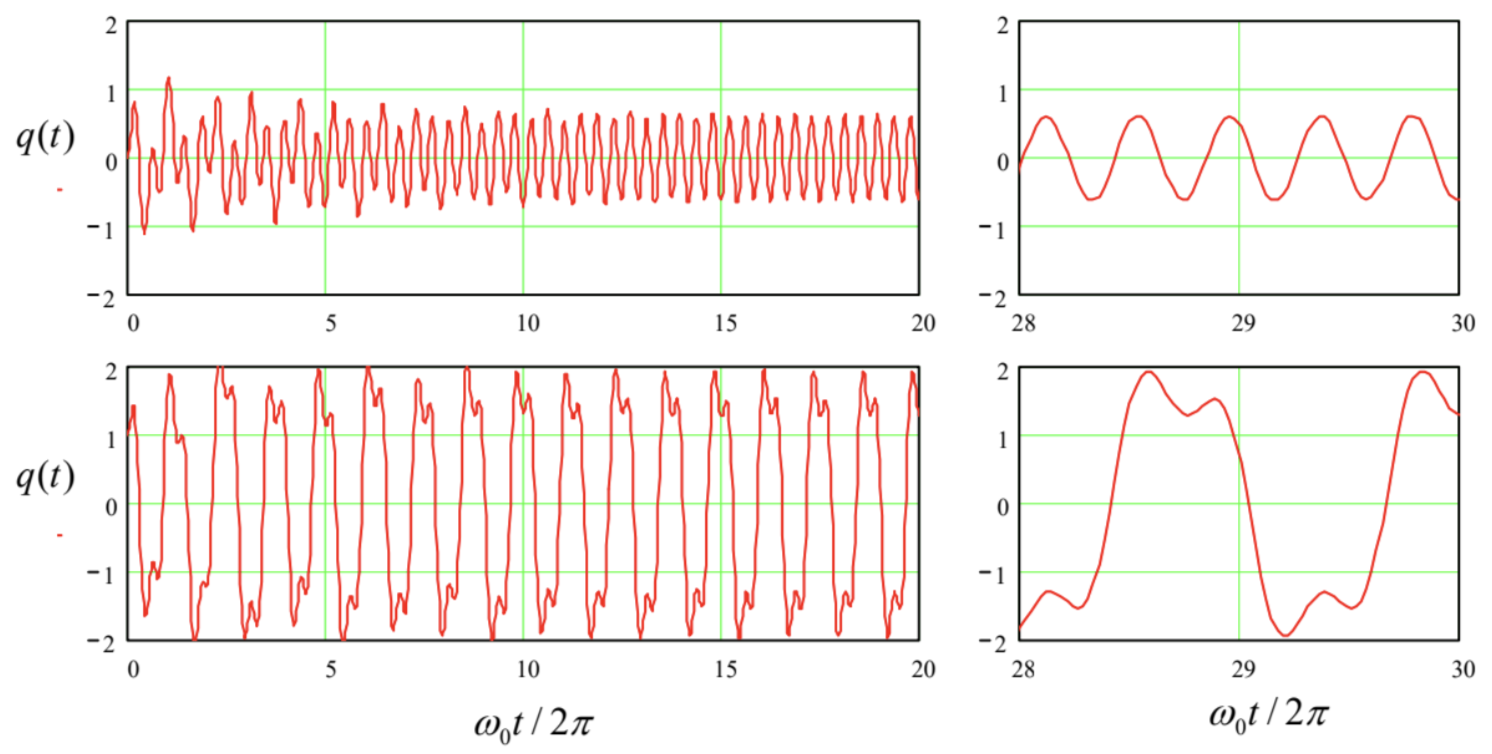
Figure 5.14. The oscillations induced in a pendulum, with damping \(\delta / \omega_{0}=0.03\), by a sinusoidal external force of amplitude \(f_{0}=0.75\), and frequencies \(\omega_{0} / 3\) (top panel) and \(0.8 \times \omega_{0} / 3\) (bottom panel).

Fig. 5.15. The oscillations of a pendulum with \(\ \delta / \omega_{0}=0.03\), driven by a sinusoidal external force of amplitude \(\ f_{0}=3\) and frequency \(\ 0.8 \times 3 \omega_{0}\), at initial conditions \(\ q(0)=0\) (the top row) and \(\ q(0)=1\) (the bottom row), with \(\ d q / d t(0)=0\) in both cases.
While the first and the last terms of the last expression depend only of the amplitudes of the individual components of oscillations, the two middle terms are more interesting, because they produce so-called combinational frequencies of the two components. For our case, the third term, \[3 A A_{\text {sub }}^{2} \cos \Psi \cos ^{2} \Psi_{\text {sub }}=\frac{3}{4} A A_{\text {sub }}^{2} \cos \left(\Psi-2 \Psi_{\text {sub }}\right)+\ldots,\] is of special importance, because it produces, besides other combinational frequencies, the subharmonic component with the total phase \[\Psi-2 \Psi_{\text {sub }}=\frac{\omega t}{3}-\varphi+2 \varphi_{\text {sub }}\] Thus, within a certain range of the mutual phase shift between the Fourier components, this nonlinear contribution is synchronous with the subharmonic oscillations, and describes the interaction that can deliver to it the energy from the external force, so that the oscillations may be sustained. Note, however, that the amplitude of the term describing this energy exchange is proportional to the square of \(A_{\text {sub }}\), and vanishes at the linearization of the equations of motion near the trivial fixed point. This means that the point is always stable, i.e., the \(3^{\text {rd }}\) subharmonic cannot be self-excited and always needs an initial "kickoff" - compare the two panels of Figure 15. The same is true for higher-order subharmonics.
Only the second subharmonic is a special case. Indeed, let us make a calculation similar to Eq. (102), by replacing Eq. (101) with \[q(t) \approx A \cos \Psi+A_{\text {sub }} \cos \Psi_{\text {sub }}, \quad \text { where } \Psi \equiv \omega t-\varphi, \quad \Psi_{\text {sub }} \equiv \frac{\omega t}{2}-\varphi_{\text {sub }},\] for a nonlinear term proportional to \(q^{2}\) : \[q^{2}=\left(A \cos \Psi+A_{\text {sub }} \cos \Psi_{\text {sub }}\right)^{2}=A^{2} \cos ^{2} \Psi+2 A A_{\text {sub }} \cos \Psi \cos \Psi_{\text {sub }}+A_{\text {sub }}^{2} \cos ^{2} \Psi_{\text {sub }} .\] Here the combinational-frequency term capable of supporting the \(2^{\text {nd }}\) subharmonic, \[2 A A_{\text {sub }} \cos \Psi \cos \Psi_{\text {sub }}=A A_{\text {sub }} \cos \left(\Psi-\Psi_{\text {sub }}\right)=A A_{\text {sub }} \cos \left(\omega t-\varphi+\varphi_{\text {sub }}\right)+\ldots,\] is linear in the subharmonic’s amplitude, i.e. survives the linearization near the trivial fixed point. This means that the second subharmonic may arise spontaneously, from infinitesimal fluctuations.
Moreover, such excitation of the second subharmonic is very similar to the parametric excitation that was discussed in detail in Sec. 5, and this similarity is not coincidental. Indeed, let us redo the expansion (106) making a somewhat different assumption - that the oscillations are a sum of the forced oscillations at the external force’s frequency \(\omega\) and an arbitrary but weak perturbation: \[q(t)=A \cos (\omega t-\varphi)+\widetilde{q}(t), \quad \text { with }|\widetilde{q}|<<A .\] Then, neglecting the small term proportional to \(\widetilde{q}^{2}\), we get \[q^{2} \approx A^{2} \cos ^{2}(\omega t-\varphi)+2 \widetilde{q}(t) A \cos (\omega t-\varphi) .\] Besides the inconsequential phase \(\varphi\), the second term in the last formula is exactly similar to the term describing the parametric effects in Eq. (75). This fact means that for a weak perturbation, a system with a quadratic nonlinearity in the presence of a strong "pumping" signal of frequency \(\omega\) is equivalent to a system with parameters changing in time with frequency \(\omega\). This fact is broadly used for the parametric excitation at high (e.g., optical) frequencies, where the mechanical means of parameter modulation (see, e.g., Figure 5) are not practicable. The necessary quadratic nonlinearity at optical frequencies may be provided by a non-centrosymmetric nonlinear crystal, e.g., the \(\beta\)-phase barium borate \(\left(\mathrm{BaB}_{2} \mathrm{O}_{4}\right)\).
Before finishing this chapter, let me elaborate a bit on a general topic: the relation between the numerical and analytical approaches to problems of dynamics - and physics as a whole. We have just seen that sometimes numerical solutions, like those shown in Figure 15b, may give vital clues for previously unanticipated phenomena such as the excitation of subharmonics. (The phenomenon of deterministic chaos, which will be discussed in Chapter 9 below, presents another example of such "numerical discoveries".) One might also argue that in the absence of exact analytical solutions, numerical simulations may be the main theoretical tool for the study of such phenomena. These hopes are, however, muted by the general problem that is frequently called the curse of dimensionality \({ }^{40}\) in which the last word refers to the number of parameters of the problem to be solved. \({ }^{41}\)
Indeed, let us have another look at Figure 15. OK, we have been lucky to find a new phenomenon, the \(3^{\text {rd }}\) subharmonic generation, for a particular set of parameters \(-\) in that case, five of them: \(\delta / \omega_{0}=\) \(0.03, \omega / \omega_{0}=2.4, f_{0}=3, q(0)=1\), and \(d q / d t(0)=0\). Could we tell anything about how common this effect is? Are subharmonics with different \(n\) possible in this system? The only way to address these questions computationally is to carry out similar numerical simulations in many points of the \(d\) dimensional (in this case, \(d=5\) ) space of parameters. Say, we have decided that breaking the reasonable range of each parameter to \(N=100\) points is sufficient. (For many problems, even more points are necessary - see, e.g., Sec. 9.1.) Then the total number of numerical experiments to carry out is \(N^{d}=\) \(\left(10^{2}\right)^{5}=10^{10}\) - not a simple task even for the powerful modern computing facilities. (Besides the pure number of required CPU cycles, consider the storage and analysis of the results.) For many important problems of nonlinear dynamics, e.g., turbulence, the parameter dimensionality \(d\) is substantially larger, and the computer resources necessary even for one numerical experiment, are much greater.
In the view of the curse of dimensionality, approximate analytical considerations, like those outlined above for the subharmonic excitation, are invaluable. More generally, physics used to stand on two legs: experiment and analytical theory. The enormous progress of computer performance during a few last decades has provided it with one more point of support (a tail? :-) - numerical simulation. This does not mean we can afford to discard any of the legs we are standing on.
\({ }^{37}\) All numerical results shown in this section have been obtained by the \(4^{\text {th }}\)-order Runge-Kutta method with the automatic step adjustment that guarantees the relative error of the order of \(10^{-4}-\) much smaller than the pixel size in the shown plots.
\({ }^{38}\) In this particular case, the higher harmonic content is about \(0.5 \%\), dominated by the \(3^{\text {rd }}\) harmonic, whose amplitude and phase are in a very good agreement with Eq. (50).
\({ }^{39}\) This method is used in practice, for example, for the generation of electromagnetic waves with frequencies in the terahertz range \(\left(10^{12}-10^{13} \mathrm{~Hz}\right)\), which still lacks efficient electronic self-oscillators that could be used as practical generators.
\({ }^{40}\) This term had been coined in 1957 by Richard Bellman in the context of the optimal control theory (where the dimensionality means the number of parameters affecting the system under control), but gradually has spread all over quantitative sciences using numerical methods.
\({ }^{41}\) In EM Sec. 1.2, I discuss implications of the curse implications for a different case, when both analytical and numerical solutions to the same problem are possible.