7.3: Hooke’s Law

In order to form a complete system of equations describing the continuum’s dynamics, one needs to complement Eq. (25) with an appropriate constitutive equation describing the relation between the forces described by the stress tensor $\sigma_{i j}$, and the deformations $\mathbf{q}$ described (in the small deformation limit) by the strain tensor $s_{j j}$. This relation depends on the medium, and generally may be rather complex. Even leaving alone various anisotropic solids (e.g., crystals) and macroscopicallyinhomogeneous materials (like ceramics or sand), strain typically depends not only on the current value of stress (possibly in a nonlinear way), but also on the previous history of stress application. Indeed, if strain exceeds a certain plasticity threshold, atoms (or nanocrystals) may slip to their new positions and never come back even if the strain is reduced. As a result, deformations become irreversible - see Figure 5 .

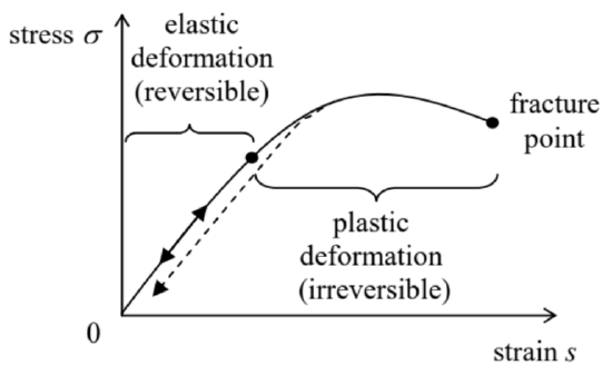Figure 7.5. A typical relation between the stress and strain in solids (schematically).

Only below the thresholds of nonlinearity and plasticity (which are typically close to each other), the strain is nearly proportional to stress, i.e. obeys the famous Hooke’s law. ${ }^{8}$ However, even in this elastic range, the law is not quite simple, and even for an isotropic medium is described not by one but by two constants, called the elastic moduli. The reason for that is that most elastic materials resist the strain accompanied by a volume change (say, the hydrostatic compression) differently from how they resist a shear deformation.

To describe this difference, let us first represent the symmetrized strain tensor $(9 b)$ in the following mathematically equivalent form: $$s_{i j^{\prime}}=\left(s_{j j^{\prime}}-\frac{1}{3} \delta_{i j^{\prime}} \operatorname{Tr}(\mathrm{s})\right)+\left(\frac{1}{3} \delta_{j j^{\prime}} \operatorname{Tr}(\mathrm{s})\right) .$$ According to Eq. (13), the traceless tensor in the first parentheses of Eq. (31) does not give any contribution to the volume change, e.g., may be used to characterize a purely shear deformation, while the second term describes the hydrostatic compression alone. Hence we may expect that the stress tensor may be represented (again, within the elastic deformation range only!) as $$\sigma_{i j^{\prime}}=2 \mu\left(s_{i j^{\prime}}-\frac{1}{3} \operatorname{Tr}(\mathrm{s}) \delta_{j j^{\prime}}\right)+3 K\left(\frac{1}{3} \operatorname{Tr}(\mathrm{s}) \delta_{j j^{\prime}}\right)$$ where $K$ and $\mu$ are constants. (The inclusion of coefficients 2 and 3 into Eq. (32) is justified by the simplicity of some of its corollaries - see, e.g., Eqs. (36) and (41) below.) Indeed, experiments show that Hooke’s law in this form is followed, at small strain, by all isotropic materials. In accordance with the above discussion, the constant $\mu$ (in some texts, denoted as $G$ ) is called the shear modulus, while the constant $K$ (sometimes denoted $B$ ), the bulk modulus. The two left columns of Table 1 show the approximate values of these moduli for typical representatives of several major classes of materials. ${ }^{9}$

Table 7.1. Elastic moduli, density, and sound velocities of a few representative materials (approximate values)

	$K(\mathrm{GPa})$	$\mu(\mathrm{GPa})$	$E(\mathrm{GPa})$	$v$	$\rho\left(\mathrm{kg} / \mathrm{m}^{3}\right)$	$v_{1}(\mathrm{~m} / \mathrm{s})$	$v_{\mathrm{t}}(\mathrm{m} / \mathrm{s})$
Diamond $^{(\mathrm{a})}$	600	450	1,100	$0.20$	3,500	1,830	1,200
Hardened steel	170	75	200	$0.30$	7,800	5,870	3,180
Water $^{(\mathrm{b})}$	$2.1$	0	0	$0.5$	1,000	1,480	0
Air $^{(\mathrm{b})}$	$0.00010$	0	0	$0.5$	$1.2$	332	0

(a) Averages over crystallographic directions ( 10% anisotropy).

(b) At the so-called ambient conditions $\left(T=20^{\circ} \mathrm{C}, P=1\right.$ bar $\left.\equiv 10^{5} \mathrm{~Pa}\right)$.

To better appreciate these values, let us first discuss the quantitative meaning of $K$ and $\mu$, using two simple examples of elastic deformation. However, in preparation for that, let us first solve the set of nine (or rather six different) linear equations (32) for $s_{j j}$. This is easy to do, due to the simple structure of these equations: they relate the components $\sigma_{i j^{\prime}}$ and $s_{i j^{\prime}}$ ’ with the same indices, besides the involvement of the tensor’s trace. This slight complication may be readily overcome by noticing that according to Eq. (32), $$\operatorname{Tr}(\sigma) \equiv \sum_{j=1}^{3} \sigma_{j j}=3 K \operatorname{Tr}(\mathrm{s}), \quad \text { so that } \operatorname{Tr}(\mathrm{s})=\frac{1}{3 K} \operatorname{Tr}(\sigma) .$$ Plugging this result into Eq. (32) and solving it for $s_{j j}$, we readily get the reciprocal relation, which may be represented in a similar form: $$s_{i j^{\prime}}=\frac{1}{2 \mu}\left(\sigma_{j j^{\prime}}-\frac{1}{3} \operatorname{Tr}(\sigma) \delta_{j j^{\prime}}\right)+\frac{1}{3 K}\left(\frac{1}{3} \operatorname{Tr}(\sigma) \delta_{j j^{\prime}}\right) .$$ Now let us apply Hooke’s law, in the form of Eqs. (32) or (34), to two simple situations in which the strain and stress tensors may be found without using the full differential equation of the elasticity theory and boundary conditions for them. (That will be the subject of the next section.) The first situation is the hydrostatic compression when the stress tensor is diagonal, and all its diagonal components are equal - see Eq. (19). ${ }^{10}$ For this case Eq. (34) yields $$s_{j j^{\prime}}=-\frac{\mathcal{P}}{3 K} \delta_{j j^{\prime}},$$ i.e. regardless of the shear modulus, the strain tensor is also diagonal, with all diagonal components equal. According to Eqs. (11) and (13), this means that all linear dimensions of the body are reduced by a similar factor, so that its shape is preserved, while the volume is reduced by $$\frac{\Delta V}{V}=\sum_{j=1}^{3} s_{j j}=-\frac{\mathcal{P}}{K} .$$ This formula clearly shows the physical sense of the bulk modulus $K$ as the reciprocal compressibility. As Table 1 shows, the values of $K$ may be dramatically different for various materials, and even for such "soft stuff" as water this modulus is actually rather high. For example, even at the bottom of the deepest, $10-\mathrm{km}$ ocean well $\left(\mathcal{P} \approx 10^{3}\right.$ bar $\left.\approx 0.1 \mathrm{GPa}\right)$, the water’s density increases by just about $5 \%$. As a result, in most human-scale experiments, water may be treated as incompressible - a condition that will be widely used in the next chapter. Many solids are even much less compressible see, for example, the first two rows of Table 1 .

Quite naturally, the most compressible media are gases. For a portion of gas, a certain background pressure $\mathcal{P}$ is necessary just for containing it within its volume $V$, so that Eq. (36) is only valid for small increments of pressure, $\Delta \mathcal{P}$ : $$\frac{\Delta V}{V}=-\frac{\Delta \mathcal{P}}{K} .$$ Moreover, the compression of gases also depends on thermodynamic conditions. (In contrast, for most condensed media, the temperature effects are very small.) For example, at ambient conditions most gases are reasonably well described by the equation of state for the model called the ideal classical gas: $$\mathcal{P} V=N k_{\mathrm{B}} T, \quad \text { i.e. } \mathcal{P}=\frac{N k_{\mathrm{B}} T}{V} .$$ where $N$ is the number of molecules in volume $V$, and $k_{\mathrm{B}} \approx 1.38 \times 10^{-23} \mathrm{~J} / \mathrm{K}$ is the Boltzmann constant. ${ }^{11}$ For a small volume change $\Delta V$ at a constant temperature $T$, this equation gives $$\left.\Delta \mathcal{P}\right|_{T=\mathrm{const}}=-\frac{N k_{\mathrm{B}} T}{V^{2}} \Delta V=-\frac{\mathcal{P}}{V} \Delta V, \quad \text { i.e. }\left.\frac{\Delta V}{V}\right|_{T=\mathrm{const}}=-\frac{\Delta \mathcal{P}}{P} .$$ Comparing this expression with Eq. (36), we get a remarkably simple result for the isothermal compression of gases, $$\left.K\right|_{T=\mathrm{const}}=\mathcal{P},$$ which means in particular that the bulk modulus listed in Table 1 is actually valid, at the ambient conditions, for almost any gas. Note, however, that the change of thermodynamic conditions (say, from isothermal to adiabatic ${ }^{12}$ ) may affect the compressibility of the gas. Now let us consider the second, rather different, fundamental experiment: a purely shear deformation shown in Figure 2. Since the traces of the matrices (15) and (20), which describe this situation, are equal to 0 , for their off-diagonal elements, Eq. (32) gives merely $\sigma_{j j}$ ’ $=2 \mu s_{j j}$, so that the deformation angle $\alpha$ (see Figure 2) is just $$\alpha=\frac{1}{\mu} \frac{F}{A} .$$ Note that the angle does not depend on the thickness $h$ of the sample, though of course the maximal linear deformation $q_{x}=\alpha h$ is proportional to the thickness. Naturally, as Table 1 shows, $\mu=0$ for all fluids, because they do not resist static shear stress.

However, not all situations, even apparently simple ones, involve just either $K$ or $\mu$. Let us consider stretching a long and thin elastic rod of a uniform cross-section of area $A$ - the so-called tensile stress experiment shown in Figure $6.13$

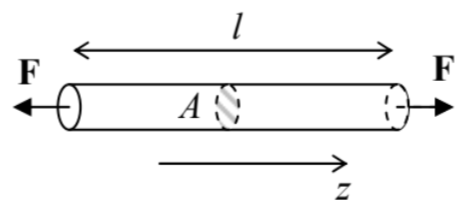Figure 7.6. The tensile stress experiment.

Though the deformation of the rod near its clamped ends depends on the exact way forces $\mathbf{F}$ are applied (we will discuss this issue later on), we may expect that over most of its length the tension forces are directed virtually along the rod, $d \mathbf{F}=F_{z} \mathbf{n}_{z}$, and hence, with the coordinate choice shown in Figure $6, \sigma_{x j}=\sigma_{y j}=0$ for all $j$, including the diagonal elements $\sigma_{x x}$ and $\sigma_{y y}$. Moreover, due to the open lateral surfaces, on which, evidently, $d F_{x}=d F_{y}=0$, there cannot be an internal stress force of any direction, acting on any elementary internal boundary parallel to these surfaces. This means that $\sigma_{z x}=$ $\sigma_{z y}=0$. So, of all components of the stress tensor only one, $\sigma_{z z}$, is not equal to zero, and for a uniform sample, $\sigma_{z z}=$ const $=F / A$. For this case, Eq. (34) shows that the strain tensor is also diagonal, but with different diagonal elements: $$\begin{gathered} s_{z z}=\left(\frac{1}{9 K}+\frac{1}{3 \mu}\right) \sigma_{z z}, \\ s_{x x}=s_{y y}=\left(\frac{1}{9 K}-\frac{1}{6 \mu}\right) \sigma_{z z} . \end{gathered}$$ Since the tensile stress is most common in engineering practice (and in physical experiment design), both combinations of the elastic moduli participating in these two relations have deserved their own names. In particular, the constant in Eq. (42) is usually denoted as $1 / E$ (but in many texts, as $1 / Y$ ), where $E$ is called Young’s modulus: 14

$$\frac{1}{E} \equiv \frac{1}{9 K}+\frac{1}{3 \mu}, \quad \text { i.e. } E \equiv \frac{9 K \mu}{3 K+\mu}$$ As Figure 6 shows, in the tensile stress geometry $s_{z z} \equiv \partial q_{z} / \partial z=\Delta l / l$ so that Young’s modulus scales the linear relation between the relative extension of the rod and the force applied per unit area: ${ }^{15}$ $$\frac{\Delta l}{l}=\frac{1}{E} \frac{F}{A} \text {. }$$ The third column of Table 1 above shows the values of this modulus for two well-known solids: diamond (with the highest known value of $E$ of all bulk materials ${ }^{16}$ ) and the steels (solid solutions of $\sim 10 \%$ of carbon in iron) used in construction. Again, for all fluids, Young’s modulus equals zero - as it follows from Eq. (44) for $\mu=0$.

I am confident that the reader of these notes has been familiar with Eq. (42), in the form of Eq. (45), from their undergraduate studies. However, most probably this cannot be said about its counterpart, Eq. (43), which shows that at the tensile stress, the rod’s cross-section dimensions also change. This effect is usually characterized by the following dimensionless Poisson’s ratio: ${ }^{17}$ $$-\frac{s_{x x}}{s_{z z}}=-\frac{s_{y y}}{s_{z z}}=-\left(\frac{1}{9 K}-\frac{1}{6 \mu}\right) /\left(\frac{1}{9 K}+\frac{1}{3 \mu}\right)=\frac{1}{2} \frac{3 K-2 \mu}{3 K+\mu} \equiv v,$$ According to this formula, for realistic materials with $K>0, \mu \geq 0, v$ may vary from (-1) to $(+1 / 2)$, but for the vast majority of materials, ${ }^{18}$ its values are between 0 and $1 / 2-$ see the corresponding column of Table 1. The lower limit of this range is reached in porous materials like cork, whose lateral dimensions almost do not change at the tensile stress. Some soft materials such as natural and synthetic rubbers present the opposite case: $v \approx 1 / 2 .{ }^{19}$ Since according to Eqs. $(13)$ and $(42)$, the volume change is $$\frac{\Delta V}{V}=s_{x x}+s_{y y}+s_{z z}=\frac{1}{E} \frac{F}{A}(1-2 v) \equiv(1-2 v) \frac{\Delta l}{l},$$ such materials virtually do not change their volume at the tensile stress. The ultimate limit of this trend, $\Delta V / V=0$, is provided by fluids and gases, because, as follows from Eq. (46) with $\mu=0$, their Poisson ratio $v$ is exactly $1 / 2$. However, for most practicable construction materials such as various steels (see Table 1) the volume change (47) is as high as $\sim 40 \%$ of that of the length.

Due to the clear physical sense of the coefficients $E$ and $v$, they are frequently used as a pair of independent elastic moduli, instead of $K$ and $\mu$. Solving Eqs. (44) and (46) for them, we get $$K=\frac{E}{3(1-2 v)}, \quad \mu=\frac{E}{2(1+v)} .$$ Using these formulas, the two (equivalent) formulations of Hooke’s law, expressed by Eqs. (32) and (34), may be rewritten as $$\begin{aligned} \sigma_{i j^{\prime}} &=\frac{E}{1+v}\left(s_{i j^{\prime}}+\frac{v}{1-2 v} \operatorname{Tr}(\mathrm{s}) \delta_{j j^{\prime}}\right) \\ s_{i j^{\prime}} &=\frac{1+v}{E}\left(\sigma_{i j^{\prime}}-\frac{v}{1+v} \operatorname{Tr}(\sigma) \delta_{i j^{\prime}}\right) \end{aligned}$$ The linear relation between the strain and stress tensor in elastic continua enables one more step in our calculation of the potential energy $U$ due to deformation, started at the end of $\mathrm{Sec} .2 .$ Indeed, to each infinitesimal part of this strain increase, we may apply Eq. (30), with the elementary work $\delta \mathscr{W}$ of the surface forces increasing the potential energy of "our" part of the body by the equal amount $\delta U$. Let us slowly increase the deformation from a completely unstrained state (in which we may take $U=0$ ) to a certain strained state, in the absence of bulk forces $\mathbf{f}$, keeping the deformation type, i.e. the relation between the elements of the stress tensor, intact. In this case, all elements of the tensor $\sigma_{i j}$ ’ are proportional to the same single parameter characterizing the stress (say, the total applied force), and according to Hooke’s law, all elements of the tensor $s_{j j}$ are proportional to that parameter as well. In this case, integration of Eq. (30) through the variation yields the following final value: 20 $$U=\int_{V} u(\mathbf{r}) d^{3} r, \quad u(\mathbf{r})=\frac{1}{2} \sum_{j, j^{\prime}=1}^{3} \sigma_{i j^{\prime}} S_{j j} .$$ Evidently, this $u(\mathbf{r})$ may be interpreted as the volumic density of the potential energy of the elastic deformation.

---

${ }^{8}$ Named after Robert Hooke (1635-1703), the polymath who was the first to describe the law in its simplest, 1D version.

${ }^{9}$ Since the strain tensor elements, defined by Eq. (9), are dimensionless, while the strain, defined by Eq. (18), has the dimensionality similar to pressure (of force per unit area), so do the elastic moduli $K$ and $\mu$.

${ }^{10}$ It may be proved that such a situation may be implemented not only in a fluid with pressure $\mathcal{P}$ but also in a solid sample of an arbitrary shape, for example by placing it into a compressed fluid.

${ }^{11}$ For the derivation and a detailed discussion of Eq. (37) see, e.g., SM Sec. 3.1.

${ }^{12}$ See, e.g., SM Sec. 1.3.

${ }^{13}$ Though the analysis of compression in this situation gives similar results, in practical experiments a strong compression of a long sample may lead to the loss of the horizontal stability - the so-called buckling - of the rod.

${ }^{14}$ Named after another polymath, Thomas Young (1773-1829) - somewhat unfairly, because his work on elasticity was predated by a theoretical analysis by L. Euler in 1727 and detailed experiments by Giordano Riccati in 1782.

${ }^{15}$ According to Eq. (47), $E$ may be thought of as the force per unit area, which would double the initial sample’s length, if only the Hooke’s law was valid for deformations that large - as it typically isn’t.

${ }^{16}$ It is probably somewhat higher (up to 2,000 GPa) in such nanostructures as carbon nanotubes and monatomic sheets (graphene), though there is still substantial uncertainty in experimentally measured elastic moduli of these structures - for a review see, e.g., G. Dimitrios et al., Prog. Mater. Sci. 90, 75 (2017).

${ }^{17}$ In some older texts, the Poisson’s ratio is denoted $\sigma$, but its notation as $v$ dominates modern literature.

${ }^{18}$ The only known exceptions are certain exotic solids with very specific internal microstructure - see, e.g., $R$. Lakes, Science 235, 1038 (1987) and references therein.

${ }^{19}$ For example, silicone rubbers (synthetic polymers broadly used in engineering and physics experiment design) have, depending on their particular composition, synthesis, and thermal curing, $v=0.47 \div 0.49$, and as a result combine respectable bulk moduli $K=(1.5 \div 2)$ GPa with very low Young’s moduli: $E=(0.0001 \div 0.05)$ GPa.

${ }^{20}$ For clarity, let me reproduce this integration for the extension of a simple 1D spring. In this case, $\delta U=\delta \mathscr{W}=$ $F \delta x$, and if the spring’s force is elastic, $F=\kappa x$, the integration yields $U=\kappa x^{2} / 2 \equiv F x / 2$.