7.2: Stress

Now let us discuss the forces that cause the strain - or, from an alternative point of view, are caused by the strain. Internal forces acting inside (i.e. between arbitrarily defined parts of) a continuum may be also characterized by a tensor. This stress tensor, \({ }^{6}\) with elements \(\sigma_{j j}\), relates the Cartesian components of the vector \(d \mathbf{F}\) of the force acting on an elementary area \(d A\) of an (in most cases, imagined) interface between two parts of a continuum, with the components of the elementary vector \(d \mathbf{A}\) \(=\mathbf{n} d A\) normal to the area \(-\) see Figure 3: \[d F_{j}=\sum_{j^{\prime}=1}^{3} \sigma_{i j^{\prime}} d A_{j^{\prime}} .\] The usual sign convention here is to take the outer normal \(d \mathbf{n}\), i.e. to direct \(d \mathbf{A}\) out of "our" part of the continuum, i.e. the part on which the calculated force \(d \mathbf{F}\) is exerted - by the complementary part.

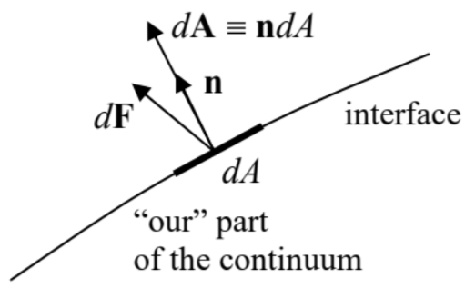
Figure 7.3. The definition of vectors \(d \mathbf{A}\) and \(d \mathbf{F}\).

In some cases, the stress tensor’s structure is very simple. For example, as will be discussed in detail in the next chapter, static and ideal fluids (i.e. liquids and gases) may only provide forces normal to any interface, and usually directed toward "our" part of the body, so that \[d \mathbf{F}=-\mathcal{P} d \mathbf{A}, \quad \text { i.e. } \sigma_{i j^{\prime}}=-\mathcal{P} \delta_{j j^{\prime}},\] where the scalar \(\mathcal{P}\) (in most cases positive) is called pressure, and generally may depend on both the spatial position and time. This type of stress, with \(\mathcal{P}>0\), is frequently called hydrostatic compressioneven if it takes place in solids, as it may.

However, in the general case, the stress tensor also has off-diagonal terms, which characterize the shear stress. For example, if the shear strain, shown in Figure 2, is caused by a pair of forces \(\pm \mathbf{F}\), they create internal forces \(F_{x} \mathbf{n}_{x}\), with \(F_{x}>0\) if we speak about the force acting upon a part of the sample below the imaginary horizontal interface we are discussing. To avoid a horizontal acceleration of each horizontal slice of the sample, the forces should not depend on \(y\), i.e. \(F_{x}=\) const \(=F\). Superficially, it may look that in this case, the only nonzero component of the stress tensor is \(d F_{x} / d A_{y}=F / A=\) const, so that tensor is asymmetric, in contrast to the strain tensor (15) of the same system. Note, however, that the pair of forces \(\pm \mathbf{F}\) creates not only the shear stress but also a nonzero rotating torque \(\tau=-F h \mathbf{n}_{z}=-\) \(\left(d F_{x} / d A_{y}\right) A h \mathbf{n}_{z}=-\left(d F_{x} / d A_{y}\right) V \mathbf{n}_{z}\), where \(V=A h\) is sample’s volume. So, if we want to perform a static stress experiment, i.e. avoid sample’s rotation, we need to apply some other forces, e.g., a pair of vertical forces creating an equal and opposite torque \(\tau^{\prime}=\left(d F_{y} / d A_{x}\right) V \mathbf{n}_{z}\), implying that \(d F_{y} / d A_{x}=d F_{x} / d A_{y}\) \(=F / A\). As a result, the stress tensor becomes symmetric, and similar in structure to the symmetrized strain tensor (15):

\[\sigma=\left(\begin{array}{ccc} 0 & F_{0} / A & 0 \\ F_{0} / A & 0 & 0 \\ 0 & 0 & 0 \end{array}\right) .\] In many situations, the body may be stressed not only by forces applied to their surfaces but also by some volume-distributed (bulk) forces \(d \mathbf{F}=\mathbf{f} d V\), whose certain effective bulk density \(\mathbf{f}\). (The most evident example of such forces is gravity. If its field is uniform as described by Eq. (1.16), then \(\mathbf{f}=\rho \mathbf{g}\), where \(\rho\) is the mass density.) Let us derive the key formula describing the summation of the interface and bulk forces. For that, consider again an elementary cuboid with sides \(d r_{j}\) parallel to the corresponding coordinate axes (Figure 4) - now not necessarily the principal axes of the stress tensor.

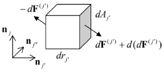Figure 7.4. Deriving Eq. (23).

If elements \(\sigma_{i j^{\prime}}\) of the tensor do not depend on position, the force \(d \mathbf{F}^{(j)}\) acting on the \(j^{\prime}\) ’-th face of the cuboid is exactly balanced by the equal and opposite force acting on its opposite face, because the vectors \(d \mathbf{A}^{\left(j^{\prime}\right)}\) at these faces are equal and opposite. However, if \(\sigma_{i j}\) is a function of \(\mathbf{r}\), then the net force \(d\left(d \mathbf{F}^{(j)}\right)\) does not vanish. (In this expression, the first differential sign refers to the elementary shift \(d r_{j}\), while the second one, to the elementary area \(d A_{j^{\prime}}\).) Using the expression \(\sigma_{i j} d A_{j}\), for to the \(j\), th contribution to the sum (18), in the first order in \(d \mathbf{r}\) the \(j^{\text {th }}\) components of the vector \(d\left(d \mathbf{F}^{(j)}\right)\) is \[d\left(d F_{j}^{\left(j^{\prime}\right)}\right)=d\left(\sigma_{i j^{\prime}} d A_{j^{\prime}}\right)=\frac{\partial \sigma_{j j^{\prime}}}{\partial r_{j^{\prime}}} d r_{j^{\prime}} d A_{j^{\prime}} \equiv \frac{\partial \sigma_{i j^{\prime}}}{\partial r_{j^{\prime}}} d V,\] where the cuboid’s volume \(d V=d r_{j} \cdot d A_{j}\) ’ evidently does not depend on the index \(j\) ’. The addition of these force components for all three pairs of cuboid faces, i.e. the summation of Eqs. (21) over all three values of the upper index \(j\) ’, yields the following relation for the \(j^{\text {th }}\) Cartesian component of the net force exerted on the cuboid: \[d\left(d F_{j}\right)=\sum_{j^{\prime}=1}^{3} d\left(d F_{j}^{\left(j^{\prime}\right)}\right)=\sum_{j^{\prime}=1}^{3} \frac{\partial \sigma_{i j^{\prime}}}{\partial r_{j^{\prime}}} d V .\] Since any volume may be broken into such infinitesimal cuboids, Eq. (22) shows that the space-varying stress is equivalent to a volume-distributed force \(d \mathbf{F}_{\text {ef }}=\mathbf{f}_{\text {ef }} d V\), whose effective (not real!) bulk density \(\mathbf{f}_{\text {ef }}\) has the following Cartesian components \[\left(f_{\text {ef }}\right)_{j}=\sum_{j^{\prime}=1}^{3} \frac{\partial \sigma_{i j^{\prime}}}{\partial r_{j^{\prime}}},\] so that in the presence of genuinely bulk forces \(d \mathbf{F}=\mathbf{f} d V\), densities \(\mathbf{f}_{\text {ef }}\) and \(\mathbf{f}\) just add up. This the socalled Euler-Cauchy stress principle.

Let us use this addition rule to spell out the \(2^{\text {nd }}\) Newton law for a unit volume of a continuum: \[\rho \frac{\partial^{2} \mathbf{q}}{\partial t^{2}}=\mathbf{f}_{\mathrm{ef}}+\mathbf{f} .\] Using Eq. (23), the \(j^{\text {th }}\) Cartesian component of Eq. (24) may be represented as \[\rho \frac{\partial^{2} q_{j}}{\partial t^{2}}=\sum_{j^{\prime}=1}^{3} \frac{\partial \sigma_{i j^{\prime}}}{\partial r_{j^{\prime}}}+f_{j} .\] This is the key equation of the continuum’s dynamics (and statics), which will be repeatedly used below.

For the solution of some problems, it is also convenient to have a general expression for the work \(\delta \mathscr{Y}\) of the stress forces at a virtual deformation \(\delta \mathbf{q}\) - understood in the same variational sense as the virtual displacements \(\delta \mathbf{r}\) in Sec. 2.1. Using the Euler-Cauchy principle (23), for any volume \(V\) of a medium not affected by volume-distributed forces, we may write \({ }^{7}\) \[\delta \mathscr{V}=-\int_{V} \mathbf{f}_{\mathrm{ef}} \cdot \delta \mathbf{q} d^{3} r=-\sum_{j=1}^{3} \int_{V}\left(f_{\mathrm{ef}}\right)_{j} \delta q_{j} d^{3} r=-\sum_{j, j^{\prime}=1}^{3} \int_{V}^{\partial \sigma_{i j^{\prime}}} \frac{\partial r_{j^{\prime}}}{\partial q_{j}} d^{3} r .\] Let us work out this integral by parts for a volume so large that the deformations \(\delta q_{j}\) on its surface are negligible. Then, swapping the operations of the variation and the spatial differentiation (just like it was done with the time derivative in Sec. 2.1), we get \[\delta \mathscr{W}=\sum_{j, j^{\prime}=1}^{3} \int_{V} \sigma_{i j^{\prime}} \delta \frac{\partial q_{j}}{\partial r_{j^{\prime}}} d^{3} r .\] Assuming that the tensor \(\sigma_{i j}\), is symmetric, we may rewrite this expression as \[\delta \mathscr{W}=\frac{1}{2} \sum_{j, j^{\prime}=1}^{3} \int_{V}\left(\sigma_{j j^{\prime}} \delta \frac{\partial q_{j}}{\partial r_{j^{\prime}}}+\sigma_{j j} \delta \frac{\partial q_{j}}{\partial r_{j^{\prime}}}\right) d^{3} r .\] Now, swapping indices \(j\) and \(j\) ’ in the second expression, we finally get \[\delta \mathscr{H}=\frac{1}{2} \sum_{j, j^{\prime}=1}^{3} \int_{V} \delta\left(\frac{\partial q_{j}}{\partial r_{j^{\prime}}} \sigma_{i j^{\prime}}+\frac{\partial q_{j^{\prime}}}{\partial r_{j}} \sigma_{j j^{\prime}}\right) d^{3} r=-\sum_{j, j^{\prime}=1}^{3} \int_{V} \sigma_{i j^{\prime}} \delta s_{j j^{\prime}} d^{3} r,\] where \(s_{j j}\) ’ are the components of the strain tensor (9b). It is natural to rewrite this important formula as \[\delta \mathscr{W}=\int_{V} \delta w(\mathbf{r}) d^{3} r, \quad \text { where } \delta w(\mathbf{r}) \equiv \sum_{j, j^{\prime}=1}^{3} \sigma_{i j^{\prime}} \delta s_{j j},\] and interpret the locally-defined scalar function \(\delta_{r c}(\mathbf{r})\) as the work of the stress forces per unit volume, at a small variation of the deformation.

As a sanity check, for the pure pressure (19), Eq. (30) is reduced to the evidently correct result \(\delta \mathscr{W}=-\mathcal{P} \delta V\), where \(V\) is the volume of "our" part of the continuum.

---

\({ }^{6}\) It is frequently called the Cauchy stress tensor, partly to honor Augustin-Louis Cauchy who introduced this notion (and is responsible for the development, mostly in the 1820s, much of the theory described in this chapter), and partly to distinguish it from and other possible definitions of the stress tensor, including the \(1^{s t}\) and \(2^{n d}\) PiolaKirchhoff tensors. For the small deformations discussed in this course, all these notions coincide.

\({ }^{7}\) Here the sign corresponds to the work of the "external" stress force \(d \mathbf{F}\), exerted on "our" part of the continuum by its counterpart - see Figure 3. Note that some texts consider the opposite definition of \(\delta \mathscr{H}\), leading to its opposite sign.