8.6: Turbulence

As Figure 15 shows, the Stokes’ result \((71)-(72)\) is only valid at \(\operatorname{Re}<<1\), while for larger values of the Reynolds number, i.e. at higher velocities \(v_{0}\), the drag force is larger. This very fact is not quite surprising, because at the derivation of the Stokes’ result, the nonlinear term \((\mathbf{v} \cdot \nabla) \mathbf{v}\) in the Navier-Stokes equation (53), which scales as \(v^{2}\), was neglected in comparison with the linear terms, scaling as \(v\). What is more surprising is that the function \(C_{\mathrm{d}}(R e)\) exhibits such a complicated behavior over many orders of velocity’s magnitude, giving a hint that the fluid flow at large Reynolds numbers should be also very complicated. Indeed, the reason for this complexity is a gradual development of very intricate, timedependent fluid patterns, called turbulence, rich with vortices - for example, see Figure 16. These vortices are especially pronounced in the region behind the moving body (the so-called wake), while the region before the body remains almost unperturbed. As Figure 15 indicates, the turbulence exhibits rather different behaviors at various velocities (i.e. values of \(\operatorname{Re}\) ), and sometimes changes rather abruptly - see, for example, the significant drag drop at \(\operatorname{Re} \approx 5 \times 10^{5}\).

In order to understand the conditions of this phenomenon, let us estimate the scale of various terms of the Navier-Stokes equation (53) for the generic case of a body with characteristic size \(l\), moving in an otherwise static, incompressible fluid, with velocity \(v\). In this case, the characteristic time scale of possible non-stationary phenomena is given by the ratio \(l / v,{ }^{41}\) so that we arrive at the following estimates: \[\begin{array}{lcccc} \text { Equation term: } & \rho \frac{\partial \mathbf{v}}{\partial t} & \rho(\mathbf{v} \cdot \nabla) \mathbf{v} & \mathbf{f} & \eta \nabla^{2} \mathbf{v} \\ \text { Order of magnitude: } & \rho \frac{v^{2}}{l} & \rho \frac{v^{2}}{l} & \rho g & \eta \frac{v}{l^{2}} \end{array}\] (I have skipped the term \(\nabla \mathcal{P}\) because as we saw in the previous section, in typical fluid flow problems it balances the viscosity term, and hence is of the same order of magnitude.) Eq. (75) shows that the relative importance of the terms may be characterized by two dimensionless ratios. \({ }^{42}\)

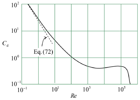
Figure 8.15. The drag coefficient \(C_{\mathrm{d}}\) for a sphere in an incompressible fluid, as a function of the Reynolds number (Note the \(\log -\log\) plot). The experimental data are from \(\mathrm{F}\). Eisner, Das Widerstandsproblem, in: Proc. \(3^{\text {rd }}\) Int. Congress on Appl. Mech., Stockholm, \(1931 .\)

The first of them is the so-called Froude number \({ }^{43}\) \[F \equiv \frac{\rho v^{2} / l}{\rho g} \equiv \frac{v^{2}}{l g},\] which characterizes the relative importance of the gravity - or, upon appropriate modification, of other bulk forces. In most practical problems (with the important exception of surface waves, see Sec. 4 above) \(F \gg>1\), so that the gravity effects may be neglected.

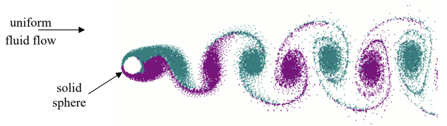
Fig. 8.16. A snapshot of the turbulent tail (wake) behind a sphere moving in a fluid with a high Reynolds number, showing the so-called von Kármán vortex street. Adapted from the original (actually, a very nice animation, http://www.mcef.ep.usp.br/staff/jmen...areo/vort2.gif) by Cesareo de La Rosa Siqueira, as a copyright-free material, available at https://commons.wikimedia.org/w/index.php?curid=87351.

Much more important is another ratio, the Reynolds number (74), which may be rewritten as \[R e \equiv \frac{\rho v l}{\eta} \equiv \frac{\rho v^{2} / l}{\eta v / l^{2}},\] and hence is a measure of the relative importance of the fluid particle’s inertia in comparison with the viscosity effects. \({ }^{44}\) So again, it is natural that for a sphere, the role of the vorticity-creating term \((\mathbf{v} \cdot \nabla) \mathbf{v}\) becomes noticeable already at \(\operatorname{Re} \sim 1-\) see Figure 15. What is very counter-intuitive is the onset of turbulence in systems where the laminar (turbulence-free) flow is formally an exact solution to the Navier-Stokes equation for any \(\operatorname{Re}\). For example, at \(\operatorname{Re}>\operatorname{Re}_{\mathrm{t}} \approx 2,100\) (with \(l \equiv 2 R\) and \(v \equiv v_{\max }\) ) the laminar flow in a round pipe, described by Eq. (60), becomes unstable, and the resulting turbulence decreases the fluid discharge \(Q\) in comparison with the Poiseuille law (62). Even more strikingly, the critical value of \(R e\) is rather insensitive to the pipe wall roughness and does not diverge even in the limit of perfectly smooth walls.

Since \(\operatorname{Re} \gg 1\) in many real-life situations, \({ }^{45}\) turbulence is very important for practice. However, despite nearly a century of intensive research, there is no general, quantitative analytical theory of this phenomenon, \({ }^{46}\) and most results are still obtained either by rather approximate analytical treatments, or by the numerical solution of the Navier-Stokes equations using the approaches discussed in the previous section, or in experiments (e.g.., on scaled models \({ }^{47}\) in wind tunnels). Only certain general, semiquantitative features may be readily understood from simple arguments.

For example, Figure 15 shows that within a very broad range of Reynolds numbers, from \(\sim 10^{2}\) to \(\sim 3 \times 10^{5}, C_{\mathrm{d}}\) of a sphere is of the order of 1 . Moreover, for a flat, thin, round disk, perpendicular to the incident flow, \(C_{\mathrm{d}}\) is very close to \(1.1\) for any \(\operatorname{Re}>10^{3}\). The approximate equality \(C_{\mathrm{d}} \approx 1\), meaning the drag force \(F \approx \rho v_{0}^{2} A / 2\), may be understood (in the picture where the object is moved by an external force \(F\) with the velocity \(v_{0}\) through a fluid which was initially at rest) as the equality of the forcedelivered power \(F v_{0}\) and the fluid’s kinetic energy \(\left(\rho v_{0}^{2} / 2\right) V\) created in volume \(V=v_{0} A\) in unit time. This relation would be exact if the object gave its velocity \(v_{0}\) to each and every fluid particle its crosssection runs into, for example by dragging all such particles behind itself. In reality, much of this kinetic energy goes into vortices, where the particle velocity may differ from \(v_{0}\), so that the equality \(C_{\mathrm{d}} \approx 1\) is only approximate.

Unfortunately, due to the time/space restrictions, for a more detailed discussion of these results I have to refer the reader to more specialized literature, \({ }^{48}\) and will conclude this chapter with a brief discussion of just one issue: can the turbulence be "explained by a single mechanism"? (In other words, can it be reduced, at least on a semi-quantitative level, to a set of simpler phenomena that are commonly considered "well understood"?) Apparently the answer is no, 49 though nonlinear dynamics of simpler systems may provide some useful insights.

At the middle of the last century, the most popular qualitative explanation of turbulence had been the formation of an "energy cascade" that would transfer the energy from the regular fluid flow to a hierarchy of vortices of various sizes. \({ }^{50}\) With our background, it is easier to retell that story in the timedomain language (with the velocity \(v\) serving as the conversion factor), using the fact that in a rotating vortex each Cartesian component of a particle’s radius-vector oscillates in time, so that to some extent the vortex plays the role of an oscillatory motion mode.

Let us consider the passage of a solid body between two, initially close, small parts of the fluid. The body pushes them apart, but after its passage, these partial volumes are free to return to their initial positions. However, the dominance of inertia effects at motion with \(\operatorname{Re}>>1\) means that the volumes continue to "oscillate" for a while about those equilibrium positions. (Since elementary volumes of an incompressible fluid cannot merge, these oscillations take the form of rotating vortices - see Figure 16 again.)

Now, from Sec. \(5.8\) we know that intensive oscillations in a system with the quadratic nonlinearity, in this case provided by the convective term \((\mathbf{v} \cdot \boldsymbol{\nabla}) \mathbf{v}\), are equivalent, for small perturbations, to the oscillation of the system’s parameters at the corresponding frequency. On the other hand, as was briefly discussed in Sec. 6.7, in a system with two oscillatory degrees of freedom, a periodic parameter change with frequency \(\omega_{\mathrm{p}}\) may lead to the non-degenerate parametric excitation ("down-conversion") of oscillations with frequencies \(\omega_{1,2}\) satisfying the relation \(\omega_{1}+\omega_{2}=\omega_{\mathrm{p}}\). Moreover, the spectrum of oscillations in such a system also has higher combinational frequencies such as \(\left(\omega_{\mathrm{p}}+\omega_{1}\right)\), thus pushing the oscillation energy up the frequency scale ("up-conversion"). In the presence of other oscillatory modes, these oscillations may in turn produce, via the same nonlinearity, even higher frequencies, etc. In a fluid, the spectrum of these "oscillatory modes" (actually, vortex structures) is essentially continuous, so that the above arguments make very plausible a sequential transfer of the energy from the moving body to a broad range of oscillatory modes - whose frequency spectrum is limited from above by the energy dissipation due to the fluid’s viscosity. When excited, these modes interact (in particular, mutually phase-lock) via the system’s nonlinearity, creating the complex motion we call turbulence.

Though not having much quantitative predictive power, such handwaving explanations, which are essentially based on the excitation of a large number of effective degrees of freedom, had been dominating the turbulence reviews until the mid-1960s. At that point, the discovery (or rather rediscovery) of quasi-random motions in classical dynamic systems with just \(a\) few degrees of freedom altered the discussion substantially. Since this phenomenon, called the deterministic chaos, extends well beyond the fluid dynamics, and I will devote to it a separate (albeit short) next chapter, and in its end will briefly return to the discussion of turbulence.

---

\({ }^{41}\) The time scale of phenomena in non-autonomous systems may be different from \(l / v\); for example, for forced oscillations of fluid flow with frequency \(\omega\), it is given by the oscillation period \(\tau \equiv 2 \pi / \omega\). For such problems, the ratio \(S \equiv(l / v) / T\) serves as another, independent dimensionless constant, commonly called either the Strouhal number or the reduced frequency.

\({ }^{42}\) For substantially compressible fluids (e.g., gases), the most important additional dimensionless parameter is the Mach number \(M \equiv v / v_{1}\), where \(v_{1}=(K / \rho)^{1 / 2}\) is the velocity of the longitudinal sound - which is, as we already know from Chapter 7 , the only wave mode possible in an infinite fluid. Especially significant for practice are supersonic effects (including the shock wave in the form of the famous Mach cone with half-angle \(\theta_{\mathrm{M}}=\sin ^{-1} M^{1}\) ) that arise at \(M>1\). For a more thorough discussion of these issues, I have to refer the reader to more specialized texts - either Chapter IX of the Landau-Lifshitz volume cited above or Chapter 15 in I. Cohen and P. Kundu, Fluid Mechanics, \(4^{\text {th }}\) ed., Academic Press, 2007 - which is generally a good book on the subject. Another popular, rather basic textbook is R. Granger, Fluid Mechanics, Dover, 1995 .

\({ }^{43}\) Named after William Froude (1810-1879) who has made several important contributions to applied hydrodynamics.

\({ }^{44}\) Note that the "dynamic" viscosity \(\eta\) participates in this number (and many other problems of fluid dynamics) only in the combination \(\eta / \rho\), which thereby has deserved a special name of kinematic viscosity.

\({ }^{45}\) Indeed, the values of \(\eta\) and \(\rho\) for water listed in Table 1 imply that even for a few-meter-sized object (such as a human body or a small boat), \(R e>1,000\) at any speed above just \(\sim 1 \mathrm{~mm} / \mathrm{s}\).

\({ }^{46}\) A rare exception is the relatively recent theoretical result by S. Orszag (1971) for the turbulence threshold in a flow of an incompressible fluid through a gap of thickness \(t\) between two parallel plane walls (see Figure 10): \(R e_{\mathrm{t}} \approx\) 5,772 (for \(l=t / 2, v=v_{\max }\) ). However, this result does not predict the turbulence patterns at \(\operatorname{Re}>\operatorname{Re}_{\mathrm{t}}\).

\({ }^{47}\) The crucial condition of correct modeling is the equality of the Reynolds numbers (74) (and if relevant, also of the Froude numbers and/or the Mach numbers) of the object of interest and its model.

\({ }^{48}\) See, e.g., P. Davidson, Turbulence, Oxford U. Press, \(2004 .\)

\({ }^{49}\) The following famous quote is attributed to Werner Heisenberg on his deathbed: "When I meet God, I will ask him two questions: Why relativity? And why turbulence? I think he will have an answer for the first question." Though probably inaccurate, this story reflects rather well the understandable frustration of the fundamental physics community, renown for their reductionist mentality, with the enormous complexity of phenomena which obey simple (e.g., the Navier-Stokes) equations, i.e. from their point of view, do not describe any new physics.

\({ }^{50}\) This picture was suggested in 1922 by Lewis F. Richardson.