8.5: Dynamics- Viscous Fluids

The viscosity of many fluids, at not overly high velocities, may be described surprisingly well by adding, to the static stress tensor (2), additional components proportional to the velocity \(\mathbf{v} \equiv d \mathbf{q} / d t\) : \[\sigma_{i j^{\prime}}=-\mathcal{P} \delta_{i j^{\prime}}+\tilde{\sigma}_{j j^{\prime}}(\mathbf{v}) .\] In the view of our experience with the Hooke’s law (7.32) expressing a stress tensor proportional to particle displacements \(\mathbf{q}\), we may expect a similar expression with the replacement \(\mathbf{q} \rightarrow \mathbf{v}=d \mathbf{q} / d t\) : \[\widetilde{\sigma}_{j j^{\prime}}=2 \eta\left(e_{j j}-\frac{1}{3} \delta_{j j^{\prime}} \operatorname{Tr}(\mathrm{e})\right)+3 \zeta\left(\frac{1}{3} \delta_{i j^{\prime}} \operatorname{Tr}(\mathrm{e})\right)\] where \(e_{i j^{\prime}}\) are the elements of the symmetrized strain derivative tensor: \[e_{i j^{\prime}} \equiv \frac{d s_{j j^{\prime}}}{d t}=\frac{1}{2}\left(\frac{\partial v_{j}}{\partial r_{j^{\prime}}}+\frac{\partial v_{j^{\prime}}}{\partial r_{j}}\right) .\] Experiment confirms that Eq. (52) gives a good description of the viscosity effects in a broad range of isotropic fluids. The coefficient \(\eta\) is called either the shear viscosity, or the dynamic viscosity, or just viscosity, while \(\zeta\) is called the second (or bulk) viscosity.

In the most frequent case of virtually incompressible fluids, \(\operatorname{Tr}(\mathrm{e})=d[\operatorname{Tr}(\mathrm{s})] / d t=(d V / d t) / V=0\), so that the term proportional to \(\zeta\) vanishes, and \(\eta\) is the only important viscosity parameter. \({ }^{29}\) Table 1 shows the approximate values of the viscosity, together with the mass density \(\rho\), for several representative fluids.

Table 8.1. Important parameters of several representative fluids (approximate values)

Fluid (all at 300 K, until indicated otherwise)	\(\eta(\mathrm{mPa} \cdot \mathrm{s})\)	\(\rho\left(\mathrm{kg} / \mathrm{m}^{3}\right)\)
Glasses	\(10^{21}-10^{24}\)	\(2,200-2,500\)
Earth magmas (at 800 to 1,400 K)	\(10^{4}-10^{14}\)	\(2,200-2,800\)
Machine oils (SAE 10W-40 W)	\(65-320\)	900
Water	\(0.89\)	1,000
Mercury	\(1.53\)	13,530
Liquid helium 4 (at 4.2K, 10 \(\mathrm{Pa}\) )	\(0.019\)	130
Air (at 10 \(\mathrm{Pa}\) )	\(0.018\)	\(1.3\)

One can see that \(\eta\) may vary in very broad limits; the extreme cases of liquids are glasses (which, somewhat counter-intuitively, are not stable solids even at room temperature, but rather may "flow", though extremely slowly, until they eventually crystallize) and liquid helium (whose viscosity is of the order of that of gases, \({ }^{30}\) despite its much higher density).

Incorporating the additional components of \(\sigma_{j j}\), to the equation \((23)\) of fluid motion, absolutely similarly to how it was done at the derivation of Eq. (7.107) of the elasticity theory, and with the account of Eq. (19), we arrive at the famous Navier-Stokes equation: \({ }^{31}\) \[\rho \frac{\partial \mathbf{v}}{\partial t}+\rho(\mathbf{v} \cdot \nabla) \mathbf{v}=-\nabla \mathcal{P}+\mathbf{f}+\eta \nabla^{2} \mathbf{v}+\left(\zeta+\frac{\eta}{3}\right) \nabla(\nabla \cdot \mathbf{v})\] The apparent simplicity of this equation should not mask an enormous range of phenomena, notably including turbulence (see the next section), that are described by it, and the complexity of its solutions even for some simple geometries. In most problems interesting for practice, the only option is to use numerical methods, but due to a large number of parameters \((\rho, \eta, \zeta\), plus geometrical parameters of the involved bodies, plus the distribution of bulk forces \(\mathbf{f}\), plus boundary conditions), this way is strongly plagued by the curse of dimensionality that was discussed in the end of Sec. 5.8.

Let us see how does the Navier-Stokes equation work, on several simple examples. As the simplest case, let us consider the so-called Couette flow of an incompressible fluid layer between two wide, horizontal plates (Figure 10), caused by their mutual sliding with a constant relative velocity \(\mathbf{v}_{0}\).

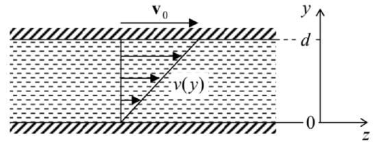Figure 8.10. The simplest problem of the viscous fluid flow.

Let us assume a laminar (vorticity-free) fluid flow. (As will be discussed in the next section, this assumption is only valid within certain limits.) Then we may use the evident symmetry of the problem, to take, in the reference frame shown in Figure \(10, \mathbf{v}=\mathbf{n}_{2} v(y)\). Let the bulk forces be vertical, \(\mathbf{f}=\mathbf{n}_{y} f\), so they do not give an additional drive to the fluid flow. Then for the stationary flow \((\partial \mathbf{v} / \partial t=0)\), the vertical, \(y\)-component of the Navier-Stokes equation is reduced to the static Pascal equation (6), showing that the pressure distribution is not affected by the plate (and fluid) motion. In the horizontal, \(z\) component of the equation, only one term, \(\nabla^{2} v\), survives, so that for the only Cartesian component of the fluid’s velocity we get the \(1 \mathrm{D}\) Laplace equation \[\frac{d^{2} v}{d y^{2}}=0 .\] In contrast to the ideal fluid (see, e.g., Figure 8b), the relative velocity of a viscous fluid and a solid wall it flows by should approach zero at the wall, \({ }^{32}\) so that Eq. (54) should be solved with boundary conditions \[v= \begin{cases}0, & \text { at } y=0, \\ v_{0}, & \text { at } y=d .\end{cases}\] Using the evident solution of this boundary problem, \(v(y)=(y / d) v_{0}\), illustrated by arrows in Figure 10, we can now calculate the horizontal drag force acting on a unit area of each plate. For the bottom plate,

\[\frac{F_{z}}{A_{y}}=\left.\sigma_{z y}\right|_{y=0}=\left.\eta \frac{\partial v}{\partial y}\right|_{y=0}=\eta \frac{v_{0}}{d} .\] (For the top plate, the derivative \(\partial v / \partial y\) has the same value, but the sign of \(d A_{y}\) has to be changed to reflect the direction of the outer normal to the solid surface so that we get a similar force but with the negative sign.) The well-known result (56) is often used, in undergraduate physics courses, for a definition of the dynamic viscosity \(\eta\), and indeed shows its meaning very well. \({ }^{33}\)

As the next, slightly less trivial example let us consider the so-called Poiseuille problem: 34 finding the relation between the constant external pressure gradient \(\chi \equiv-\partial \mathcal{P} / \partial z\) applied along a round pipe with internal radius \(R\) (Figure 11), and the so-called discharge \(Q\) - defined as the mass of fluid flowing through the pipe’s cross-section in unit time.

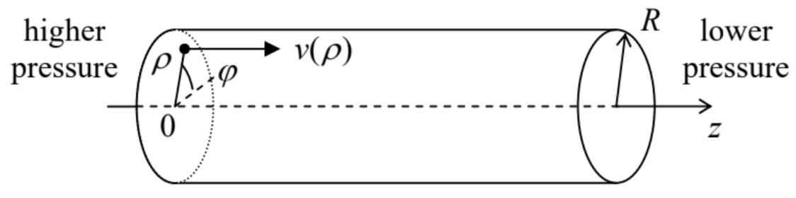Figure 8.11. The Poiseuille problem.

Again assuming a laminar flow, we can involve the problem’s uniformity along the \(z\)-axis and its axial symmetry to infer that \(\mathbf{v}=\mathbf{n}_{z} v(\rho)\), and \(\mathcal{P}=-\chi z+f(\rho, \varphi)+\operatorname{const}\) (where \(\rho=\{\rho, \varphi\}\) is again the 2D radius-vector rather than the fluid density), so that the Navier-Stokes equation (53) for an incompressible fluid (with \(\nabla \cdot \mathbf{v}=0\) ) is reduced to the following 2D Poisson equation: \[\eta \nabla_{2}^{2} v=-\chi\] After spelling out the \(2 \mathrm{D}\) Laplace operator in polar coordinates for our axially-symmetric case \(\partial / \partial \varphi=0\), Eq. (57) becomes a simple ordinary differential equation, \[\eta \frac{1}{\rho} \frac{d}{d \rho}\left(\rho \frac{d v}{d \rho}\right)=-\chi,\] which has to be solved on the segment \(0 \leq \rho \leq R\), with the following boundary conditions: \[\begin{aligned} &v=0, \quad \text { at } \rho=R, \\ &\frac{d v}{d \rho}=0, \quad \text { at } \rho=0 . \end{aligned}\] (The latter condition is required by the axial symmetry.) A straightforward double integration yields: \[v=\frac{\chi}{4 \eta}\left(R^{2}-\rho^{2}\right),\] so that the (easy) integration of the mass flow density over the cross-section of the pipe, \[Q \equiv \int_{A} \rho v d^{2} r=2 \pi \rho \frac{\chi}{4 \eta} \int_{0}^{R}\left(R^{2}-\rho^{\prime 2}\right) \rho^{\prime} d \rho^{\prime},\] immediately gives us the so-called Poiseuille (or "Hagen-Poiseuille") law for the fluid discharge: \[Q=\frac{\pi}{8} \rho \frac{\chi}{\eta} R^{4}\] where (sorry!) \(\rho\) is the mass density again. The most prominent (and practically important) feature of this result is the very strong dependence of the discharge on the pipe’s radius.

Of course, not for each cross-section shape the 2D Poisson equation (57) is so readily solvable. For example, consider a very simple, square-shape cross-section with side \(a\) (Figure 12). In this case, it is natural to use the Cartesian coordinates, so that Eq. (57) becomes \[\frac{\partial^{2} v}{\partial x^{2}}+\frac{\partial^{2} v}{\partial y^{2}}=-\frac{\chi}{\eta}=\text { const, } \quad \text { for } 0 \leq x, y \leq a,\] and (for the coordinate choice shown in Figure 12) has to be solved with boundary conditions \[v=0, \quad \text { at } x, y=0, a .\] 

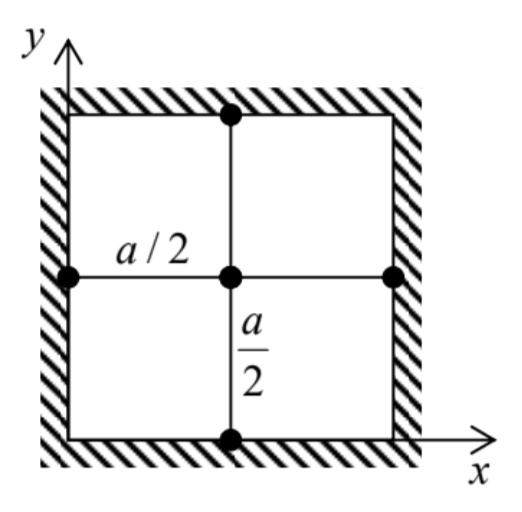
Figure 8.12. Application of the finitedifference method with a very coarse mesh (with step \(h=a / 2\) ) to the problem of viscous fluid flow in a pipe with a square cross-section.

For this boundary problem, analytical methods such as the variable separation give answers in the form of infinite sums (series), \({ }^{35}\) which ultimately require computers anyway - for their plotting and comprehension. Let me use this pretext to discuss how explicitly numerical methods may be used for such problems - or for any partial differential equations involving the Laplace operator. The simplest of them is the finite-difference method \(^{36}\) in which the function to be calculated, \(f(\mathbf{r})\), is represented by its values \(f\left(\mathbf{r}_{1}\right), f\left(\mathbf{r}_{2}\right), \ldots\) in discrete points of a rectangular grid (frequently called the mesh) of the corresponding dimensionality (Figure 13).

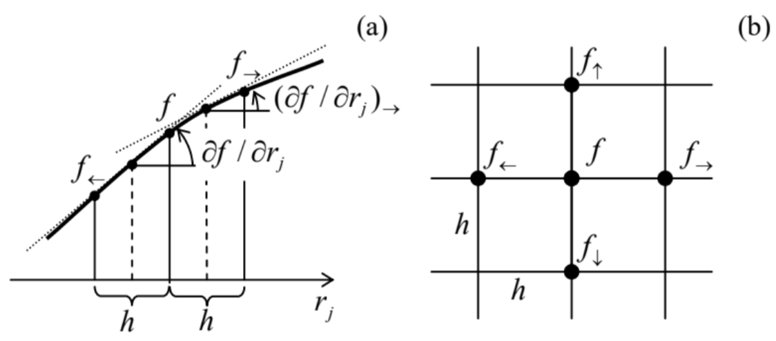Figure 8.13. The idea of the finitedifference method in (a) one and (b) two dimensions.

In Sec. 5.7, we have already discussed how to use such a grid to approximate the first derivative of the function - see Eq. (5.97). Its extension to the second derivative is straightforward - see Figure 13a:37 \[\frac{\partial^{2} f}{\partial r_{j}^{2}} \equiv \frac{\partial}{\partial r_{j}}\left(\frac{\partial f}{\partial r_{j}}\right) \approx \frac{1}{h}\left(\left.\frac{\partial f}{\partial r_{j}}\right|_{\rightarrow}-\left.\frac{\partial f}{\partial r_{j}}\right|_{\leftarrow}\right) \approx \frac{1}{h}\left[\frac{f_{\rightarrow}-f}{h}-\frac{f-f_{\leftarrow}}{h}\right] \equiv \frac{f_{\rightarrow}+f_{\leftarrow}-2 f}{h^{2}} .\] The relative error of this approximation is of the order of \(h^{2} \partial^{4} f / \partial r_{j}^{4}\), quite acceptable in many cases. As a result, the left-hand side of Eq. (63), treated on a square mesh with step \(h\) (Figure 13b), may be approximated with the so-called five-point scheme: \[\frac{\partial^{2} v}{\partial x^{2}}+\frac{\partial^{2} v}{\partial y^{2}} \approx \frac{v_{\rightarrow}+v_{\leftarrow}-2 v}{h^{2}}+\frac{v_{\uparrow}+v_{\downarrow}-2 v}{h^{2}}=\frac{v_{\rightarrow}+v_{\leftarrow}+v_{\uparrow}+v_{\downarrow}-4 v}{h^{2}} .\] (The generalization to the seven-point scheme, appropriate for 3D problems, is straightforward.) Let us apply this scheme to the pipe with the square cross-section, using an extremely coarse mesh with step \(h\) \(=a / 2\) (Figure 12). In this case, the fluid velocity \(v\) should equal zero at the walls, i.e. in all points of the five-point scheme except for the central point (in which the velocity is evidently the largest), so that Eqs. (63) and (66) yield 38 \[\frac{0+0+0+0-4 v_{\max }}{(a / 2)^{2}} \approx-\frac{\chi}{\eta}, \quad \text { i.e. } v_{\max } \approx \frac{1}{16} \frac{\chi a^{2}}{\eta}\] This result for the maximal velocity is only \(\sim 20 \%\) different from the exact value. Using a slightly finer mesh with \(h=a / 4\), which gives a readily solvable system of three linear equations for three different velocity values (the exercise left for the reader), brings us within just a couple of percent from the exact result. So such numerical methods may be practically more efficient than the "analytical" ones, even if the only available tool is a calculator app on your smartphone rather than an advanced computer.

Of course, many practical problems of fluid dynamics do require high-performance computing, especially in conditions of turbulence (see the next section) with its complex, irregular spatial-temporal structure. In these conditions, the finite-difference approach discussed above may become unsatisfactory, because it implies the same accuracy of the derivative approximation through the whole area of interest. A more powerful (but also much more complex for implementation) approach is the finite-element method in which the discrete-point mesh is based on triangles with uneven sides, and is (in most cases, automatically) generated in accordance with the system geometry, giving many more mesh points at the location(s) of the highest gradients of the calculated function (Figure 14), and hence a better calculation accuracy for the same total number of points. Unfortunately, I do not have time for going into the details of that method, so the interested reader is referred to the special literature on this subject. \({ }^{39}\)

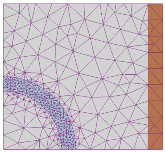
Figure 8.14. A typical finite-element mesh generated automatically for a system with relatively complex geometry - a round cylindrical shell inside another one, with mutually perpendicular axes. (Adapted from the original by I. Zureks, https://commons.wikimedia.org/w/in dex.php?curid \(=2358783\), under the CC license BY-SA 3.0.)

Before proceeding to our next topic, let me mention one more important problem that is analytically solvable using the Navier-Stokes equation: a slow motion of a solid sphere of radius \(R\), with a constant velocity \(\mathbf{v}_{0}\), through an incompressible viscous fluid - or equivalently, a slow flow of the fluid (uniform at large distances) around an immobile sphere. Indeed, in the limit \(v \rightarrow 0\), the second term on the left-hand side of Eq. (53) is negligible (just as at the surface wave analysis in Sec. 3), and the equation takes the form \[-\nabla \mathcal{P}+\eta \nabla^{2} \mathbf{v}=0,\] which should be complemented with the incompressibility condition \(\nabla \cdot \mathbf{v}=0\) and boundary conditions \[\begin{aligned} &\mathbf{v}=0, \quad \text { at } r=R, \\ &\mathbf{v} \rightarrow \mathbf{v}_{0}, \text { at } r \rightarrow \infty . \end{aligned}\] In spherical coordinates, with the polar axis directed along the vector \(\mathbf{v}_{0}\), this boundary problem has the axial symmetry (so that \(\partial \mathbf{v} / \partial \varphi=0\) and \(v_{\varphi}=0\) ), and allows the following analytical solution: \[v_{r}=v_{0} \cos \theta\left(1-\frac{3 R}{2 r}+\frac{R^{3}}{2 r^{2}}\right), \quad v_{\theta}=-v_{0} \sin \theta\left(1-\frac{3 R}{4 r}-\frac{R^{3}}{4 r^{2}}\right) .\] Calculating the pressure distribution from Eq. (68), and integrating it over the surface of the sphere, it is now straightforward to obtain the famous Stokes formula for the drag force acting on the sphere: \[F=6 \pi \eta R v_{0} .\] Historically, this formula has played an important role in the first precise (better than \(1 \%\) ) calculation of the fundamental electric charge \(e\) by R. Millikan and H. Fletcher from their famous oil drop experiments in 1909-1913.

For what follows in the next section, it is convenient to recast this result into the following form: \[C_{\mathrm{d}}=\frac{24}{R e},\] where \(C_{\mathrm{d}}\) is the drag coefficient defined as \[C_{\mathrm{d}} \equiv \frac{F}{\rho v_{0}^{2} A / 2},\] with \(A \equiv \pi R^{2}\) being the sphere’s cross-section "as seen by the incident fluid flow", and \(\operatorname{Re}\) is the socalled Reynolds number. \({ }^{40}\) In the general case, the number is defined as \[\operatorname{Re} \equiv \frac{\rho v l}{\eta},\] where \(l\) is the linear-size scale of the problem, and \(v\) is its velocity scale. (In the particular case of Eq. (72) for the sphere, \(l\) is identified with the sphere’s diameter \(D=2 R\), and \(v\) with \(v_{0}\) ). The physical sense of these two definitions will be discussed in the next section.

---

\({ }^{29}\) Probably the most important effect we miss by neglecting \(\zeta\) is the attenuation of the (longitudinal) acoustic waves, into which the second viscosity makes a major (and in some cases, the main) contribution - whose (rather straightforward) analysis is left for the reader’s exercise.

\({ }^{30}\) Actually, at even lower temperatures (for \(\mathrm{He} 4\), at \(T<T_{\lambda} \approx 2.17 \mathrm{~K}\) ), helium becomes a superfluid, i.e. loses its viscosity completely, as a result of the Bose-Einstein condensation - see, e.g., SM Sec. 3.4.

\({ }^{31}\) Named after Claude-Louis Navier (1785-1836) who had suggested the equation, and Sir George Gabriel Stokes (1819-1903) who has demonstrated its relevance by solving the equation for several key situations.

\({ }^{32}\) This is essentially an additional experimental fact, but may be understood as follows. The tangential component of the velocity should be continuous at the interface between two viscous fluids, in order to avoid infinite stress see Eq. (52), and solid may be considered as an ultimate case of fluid, with infinite viscosity.

\({ }^{33}\) The very notion of viscosity \(\eta\) was introduced (by nobody other than the same Sir Isaac Newton) via a formula similar to Eq. (56), so that any effect resulting in a drag force proportional to velocity is frequently called the Newtonian viscosity.

\({ }^{34}\) It was solved by G. Stokes in 1845 to explain the experimental results obtained by Gotthilf Hagen in 1839 and (independently) by Jean Poiseuille in 1840-41.

\({ }^{35}\) See, e.g., EM Sec. \(2.5\).

\({ }^{36}\) For more details see, e.g., R. Leveque, Finite Difference Methods for Ordinary and Partial Differential Equations, SIAM, \(2007 .\)

\({ }^{37}\) As a reminder, at the beginning of Sec. \(6.4\) we have already discussed the reciprocal transition - from a similar sum to the second derivative in the continuous limit \((h \rightarrow 0)\).

\({ }^{38}\) Note that value (67) of \(v_{\max }\) is exactly the same as given by the analytical formula (60) for the round crosssection with the radius \(R=a / 2\). This is not an occasional coincidence. The velocity distribution given by (60) is a quadratic function of both \(x\) and \(y\). For such functions, with all derivatives higher than \(\partial^{2} f / \partial r_{j}^{2}\) equal to zero, equation (66) is exact rather than approximate.

\({ }^{39}\) I can recommend, e.g., C. Johnson, Numerical Solution of Partial Differential Equations by the Finite Element Method, Dover, 2009, or T. Hughes, The Finite Element Method, Dover, \(2000 .\)

\({ }^{40}\) This notion was introduced in 1851 by the same G. Stokes but eventually named after O. Reynolds who popularized it three decades later.