
9.1: Chaos in Maps
- Page ID
- 34804

\( \newcommand{\vecs}[1]{\overset { \scriptstyle \rightharpoonup} {\mathbf{#1}} } \)
\( \newcommand{\vecd}[1]{\overset{-\!-\!\rightharpoonup}{\vphantom{a}\smash {#1}}} \)
\( \newcommand{\dsum}{\displaystyle\sum\limits} \)
\( \newcommand{\dint}{\displaystyle\int\limits} \)
\( \newcommand{\dlim}{\displaystyle\lim\limits} \)
\( \newcommand{\id}{\mathrm{id}}\) \( \newcommand{\Span}{\mathrm{span}}\)
( \newcommand{\kernel}{\mathrm{null}\,}\) \( \newcommand{\range}{\mathrm{range}\,}\)
\( \newcommand{\RealPart}{\mathrm{Re}}\) \( \newcommand{\ImaginaryPart}{\mathrm{Im}}\)
\( \newcommand{\Argument}{\mathrm{Arg}}\) \( \newcommand{\norm}[1]{\| #1 \|}\)
\( \newcommand{\inner}[2]{\langle #1, #2 \rangle}\)
\( \newcommand{\Span}{\mathrm{span}}\)
\( \newcommand{\id}{\mathrm{id}}\)
\( \newcommand{\Span}{\mathrm{span}}\)
\( \newcommand{\kernel}{\mathrm{null}\,}\)
\( \newcommand{\range}{\mathrm{range}\,}\)
\( \newcommand{\RealPart}{\mathrm{Re}}\)
\( \newcommand{\ImaginaryPart}{\mathrm{Im}}\)
\( \newcommand{\Argument}{\mathrm{Arg}}\)
\( \newcommand{\norm}[1]{\| #1 \|}\)
\( \newcommand{\inner}[2]{\langle #1, #2 \rangle}\)
\( \newcommand{\Span}{\mathrm{span}}\) \( \newcommand{\AA}{\unicode[.8,0]{x212B}}\)
\( \newcommand{\vectorA}[1]{\vec{#1}} % arrow\)
\( \newcommand{\vectorAt}[1]{\vec{\text{#1}}} % arrow\)
\( \newcommand{\vectorB}[1]{\overset { \scriptstyle \rightharpoonup} {\mathbf{#1}} } \)
\( \newcommand{\vectorC}[1]{\textbf{#1}} \)
\( \newcommand{\vectorD}[1]{\overrightarrow{#1}} \)
\( \newcommand{\vectorDt}[1]{\overrightarrow{\text{#1}}} \)
\( \newcommand{\vectE}[1]{\overset{-\!-\!\rightharpoonup}{\vphantom{a}\smash{\mathbf {#1}}}} \)
\( \newcommand{\vecs}[1]{\overset { \scriptstyle \rightharpoonup} {\mathbf{#1}} } \)
\(\newcommand{\longvect}{\overrightarrow}\)
\( \newcommand{\vecd}[1]{\overset{-\!-\!\rightharpoonup}{\vphantom{a}\smash {#1}}} \)
\(\newcommand{\avec}{\mathbf a}\) \(\newcommand{\bvec}{\mathbf b}\) \(\newcommand{\cvec}{\mathbf c}\) \(\newcommand{\dvec}{\mathbf d}\) \(\newcommand{\dtil}{\widetilde{\mathbf d}}\) \(\newcommand{\evec}{\mathbf e}\) \(\newcommand{\fvec}{\mathbf f}\) \(\newcommand{\nvec}{\mathbf n}\) \(\newcommand{\pvec}{\mathbf p}\) \(\newcommand{\qvec}{\mathbf q}\) \(\newcommand{\svec}{\mathbf s}\) \(\newcommand{\tvec}{\mathbf t}\) \(\newcommand{\uvec}{\mathbf u}\) \(\newcommand{\vvec}{\mathbf v}\) \(\newcommand{\wvec}{\mathbf w}\) \(\newcommand{\xvec}{\mathbf x}\) \(\newcommand{\yvec}{\mathbf y}\) \(\newcommand{\zvec}{\mathbf z}\) \(\newcommand{\rvec}{\mathbf r}\) \(\newcommand{\mvec}{\mathbf m}\) \(\newcommand{\zerovec}{\mathbf 0}\) \(\newcommand{\onevec}{\mathbf 1}\) \(\newcommand{\real}{\mathbb R}\) \(\newcommand{\twovec}[2]{\left[\begin{array}{r}#1 \\ #2 \end{array}\right]}\) \(\newcommand{\ctwovec}[2]{\left[\begin{array}{c}#1 \\ #2 \end{array}\right]}\) \(\newcommand{\threevec}[3]{\left[\begin{array}{r}#1 \\ #2 \\ #3 \end{array}\right]}\) \(\newcommand{\cthreevec}[3]{\left[\begin{array}{c}#1 \\ #2 \\ #3 \end{array}\right]}\) \(\newcommand{\fourvec}[4]{\left[\begin{array}{r}#1 \\ #2 \\ #3 \\ #4 \end{array}\right]}\) \(\newcommand{\cfourvec}[4]{\left[\begin{array}{c}#1 \\ #2 \\ #3 \\ #4 \end{array}\right]}\) \(\newcommand{\fivevec}[5]{\left[\begin{array}{r}#1 \\ #2 \\ #3 \\ #4 \\ #5 \\ \end{array}\right]}\) \(\newcommand{\cfivevec}[5]{\left[\begin{array}{c}#1 \\ #2 \\ #3 \\ #4 \\ #5 \\ \end{array}\right]}\) \(\newcommand{\mattwo}[4]{\left[\begin{array}{rr}#1 \amp #2 \\ #3 \amp #4 \\ \end{array}\right]}\) \(\newcommand{\laspan}[1]{\text{Span}\{#1\}}\) \(\newcommand{\bcal}{\cal B}\) \(\newcommand{\ccal}{\cal C}\) \(\newcommand{\scal}{\cal S}\) \(\newcommand{\wcal}{\cal W}\) \(\newcommand{\ecal}{\cal E}\) \(\newcommand{\coords}[2]{\left\{#1\right\}_{#2}}\) \(\newcommand{\gray}[1]{\color{gray}{#1}}\) \(\newcommand{\lgray}[1]{\color{lightgray}{#1}}\) \(\newcommand{\rank}{\operatorname{rank}}\) \(\newcommand{\row}{\text{Row}}\) \(\newcommand{\col}{\text{Col}}\) \(\renewcommand{\row}{\text{Row}}\) \(\newcommand{\nul}{\text{Nul}}\) \(\newcommand{\var}{\text{Var}}\) \(\newcommand{\corr}{\text{corr}}\) \(\newcommand{\len}[1]{\left|#1\right|}\) \(\newcommand{\bbar}{\overline{\bvec}}\) \(\newcommand{\bhat}{\widehat{\bvec}}\) \(\newcommand{\bperp}{\bvec^\perp}\) \(\newcommand{\xhat}{\widehat{\xvec}}\) \(\newcommand{\vhat}{\widehat{\vvec}}\) \(\newcommand{\uhat}{\widehat{\uvec}}\) \(\newcommand{\what}{\widehat{\wvec}}\) \(\newcommand{\Sighat}{\widehat{\Sigma}}\) \(\newcommand{\lt}{<}\) \(\newcommand{\gt}{>}\) \(\newcommand{\amp}{&}\) \(\definecolor{fillinmathshade}{gray}{0.9}\)The possibility of quasi-random dynamics of deterministic systems with a few degrees of freedom (nowadays called the deterministic chaos - or just "chaos") had been noticed before the \(20^{\text {th }}\) century, \({ }^{1}\) but has become broadly recognized only after the publication of a 1963 paper by theoretical meteorologist Edward Lorenz. In that work, he examined numerical solutions of the following system of three nonlinear, ordinary differential equations, \[\begin{aligned} \dot{q}_{1} &=a_{1}\left(q_{2}-q_{1}\right) \\ \dot{q}_{2} &=a_{2} q_{1}-q_{2}-q_{1} q_{3}, \\ \dot{q}_{3} &=q_{1} q_{2}-a_{3} q_{3}, \end{aligned}\] as a rudimentary model of heat transfer through a horizontal layer of fluid separating two solid plates. (Experiment shows that if the bottom plate is kept hotter than the top one, the liquid may exhibit turbulent convection.) He has found that within a certain range of the constants \(a_{1,2,3}\), the solution to Eq. (1) follows complex, unpredictable, non-repeating trajectories in the 3D \(q\)-space. Moreover, the functions \(q_{j}(t)\) (where \(j=1,2,3\) ) are so sensitive to initial conditions \(q_{j}(0)\) that at sufficiently large times \(t\), solutions corresponding to slightly different initial conditions become completely different.
Very soon it was realized that such behavior is typical for even simpler mathematical objects called maps so that I will start my discussion of chaos from these objects. A 1D map is essentially a rule for finding the next number \(q_{n+1}\) of a discrete sequence numbered by the integer index \(n\), in the simplest cases using only its last known value \(q_{n}\). The most famous example is the so-called \(\operatorname{logistic}\) map: \(^{2}\) \[q_{n+1}=f\left(q_{n}\right) \equiv r q_{n}\left(1-q_{n}\right) .\] The basic properties of this map may be understood using the (hopefully, self-explanatory) graphical representation shown in Figure 1. \({ }^{3}\) One can readily see that at \(r<1\) (Figure 1a) the logistic map sequence rapidly converges to the trivial fixed point \(q^{(0)}=0\), because each next value of \(q\) is less than the previous one. However, if \(r\) is increased above 1 (as in the example shown in Figure 1b), the fixed point \(q^{(0)}\) becomes unstable. Indeed, at \(q_{n}<<1\), the map yields \(q_{n+1} \approx r q_{n}\), so that at \(r>1\), the values \(q_{n}\) grow with each iteration. Instead of the unstable point \(q^{(0)}=0\), in the range \(1<r<r_{1}\), where \(r_{1} \equiv 3\), the map has a stable fixed point \(q^{(1)}\) that may be found by plugging this value into both parts of Eq. (2): \[q^{(1)}=f\left(q^{(1)}\right) \equiv r q^{(1)}\left(1-q^{(1)}\right),\] giving \(q^{(1)}=1-1 / r-\) see the left branch of the plot shown in Figure \(2 .\)
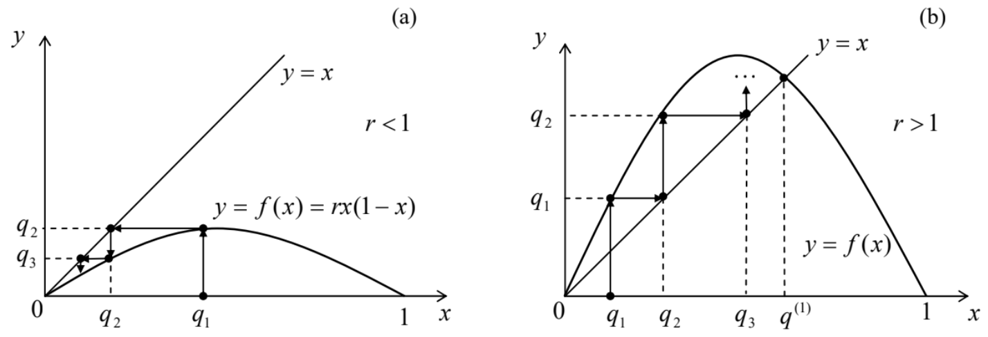
Figure 9.1. Graphical analysis of the logistic map for: (a) \(r<1\) and (b) \(r>1\).
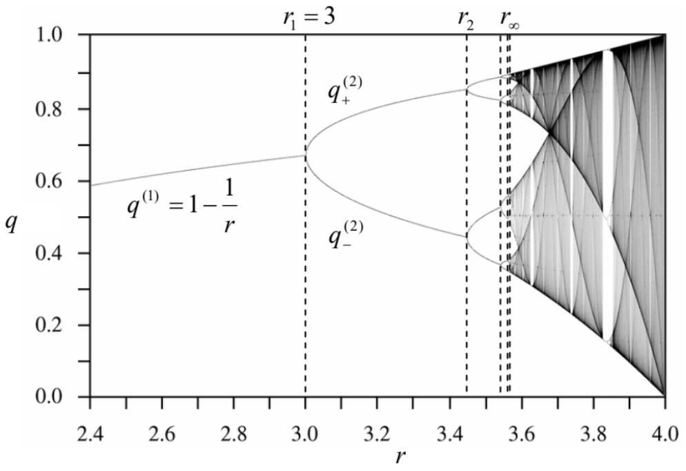 Figure 9.2. The fixed points and chaotic regions of the logistic map. Adapted, under the CCO 1.0 Universal Public Domain Dedication, from the original by Jordan Pierce, available at http://en.wikipedia.org/wiki/Logistic_map. (A very nice live simulation of the map is also available on this website.)
However, at \(r>r_{1}=3\), the fixed point \(q^{(1)}\) also becomes unstable. To prove that, let us take
\(q_{n} \equiv q^{(1)}+\widetilde{q}_{n}\), assume that the deviation \(\widetilde{q}_{n}\) from the fixed point \(q^{(1)}\) is small, and linearize the map (2)
in \(\widetilde{q}_{n}-\) just as we repeatedly did for differential equations earlier in this course. The result is \[\widetilde{q}_{n+1}=\left.\frac{d f}{d q}\right|_{q=q^{(1)}} \widetilde{q}_{n}=r\left(1-2 q^{(1)}\right) \widetilde{q}_{n}=(2-r) \widetilde{q}_{n} .\] To prove that, let us take \[\widetilde{q}_{n+1}=\left.\frac{d f}{d q}\right|_{q=q^{(1)}} \tilde{q}_{n}=r\left(1-2 q^{(1)}\right) \widetilde{q}_{n}=(2-r) \widetilde{q}_{n} .\] It shows that at \(0<2-r<1\), i.e. at \(1<r<2\), the deviations \(\widetilde{q}_{n}\) decrease monotonically. At \(-1<2-r\) \(<0\), i.e. in the range \(2<r<3\), the deviations’ sign alternates, but their magnitude still decreases \(-\) as in a stable focus, see Sec. 5.6. However, at \(-1<2-r\), i.e. \(r>r_{1} \equiv 3\), the deviations grow by magnitude, while still changing their sign, at each step. Since Eq. (2) has no other fixed points, this means that at \(n\) \(\rightarrow \infty\), the values \(q_{n}\) do not converge to one point; rather, within the range \(r_{1}<r<r_{2}\), they approach a limit cycle of alternation of two points, \(q_{+}{ }^{(2)}\) and \(q_{-}{ }^{(2)}\), which satisfy the following system of algebraic equations: \[q_{+}^{(2)}=f\left(q_{-}^{(2)}\right), \quad q_{-}^{(2)}=f\left(q_{+}^{(2)}\right) .\] These points are also plotted in Figure 2, as functions of the parameter \(r\). What has happened at the point \(r_{1}\) \(=3\) is called the period-doubling bifurcation.
The story repeats at \(r=r_{2} \equiv 1+\sqrt{6} \approx 3.45\), where the system goes from the 2 -point limit cycle to a 4-point cycle, then at \(r=r_{3} \approx 3.54\), where the limit cycle becomes consisting of 8 alternating points, etc. Most remarkably, the period-doubling bifurcation points \(r_{n}\), at that the number of points in the limit cycle doubles from \(2^{n-1}\) points to \(2^{n}\) points, become closer and closer. Numerical calculations show that at \(n \rightarrow \infty\), these points obey the following asymptotic behavior: \[r_{n} \rightarrow r_{\infty}-\frac{C}{\delta^{n}}, \text { where } r_{\infty}=3.5699 \ldots, \quad \delta=4.6692 \ldots\] The parameter \(\delta\) is called the Feigenbaum constant; for other maps, and some dynamic systems (see the next section), period-doubling sequences follow a similar law, but with different values of \(\delta\).
More important for us, however, is what happens at \(r>r_{\infty} .\) Numerous numerical experiments, repeated with increasing precision, \({ }^{4}\) have confirmed that here the system is fully disordered, with no reproducible limit cycle, though (as Figure 2 shows) at \(r \approx r_{\infty}\), all sequential values \(q_{n}\) are still confined to a few narrow regions. \({ }^{5}\) However, as parameter \(r\) is increased well beyond \(r_{\infty}\), these regions broaden and merge. This is the so-called deep chaos, with no apparent order at all. \({ }^{6}\)
The most important feature of the chaos (in this and any other system) is the exponential divergence of trajectories. For a 1D map, this means that even if the initial conditions \(q_{1}\) in two map implementations differ by a very small amount \(\Delta q_{1}\), the difference \(\Delta q_{n}\) between the corresponding sequences \(q_{n}\) is growing, on average, exponentially with \(n\). Such exponents may be used to characterize chaos. Indeed, an evident generalization of Eq. (4) to an arbitrary point \(q_{n}\) is \[\Delta q_{n+1}=e_{n} \Delta q_{n},\left.\quad e_{n} \equiv \frac{d f}{d q}\right|_{q=q_{n}} .\] Let us assume that \(\Delta q_{1}\) is so small that \(N\) first values \(q_{n}\) are relatively close to each other. Then using Eq. (7) iteratively for these steps, we get \[\Delta q_{N}=\Delta q_{1} \prod_{n=1}^{N} e_{n}, \quad \text { so that } \ln \left|\frac{\Delta q_{N}}{\Delta q_{1}}\right|=\sum_{n=1}^{N} \ln \left|e_{n}\right| \text {. }\] Numerical experiments show that in most chaotic regimes, at \(N \rightarrow \infty\) such a sum fluctuates about an average, which grows as \(\lambda N\), with the parameter \[\lambda \equiv \lim _{\Delta q_{1} \rightarrow 0} \lim _{N \rightarrow \infty} \frac{1}{N} \sum_{n=1}^{N} \ln \left|e_{n}\right|,\] called the Lyapunov exponent \({ }^{7}\) being independent of the initial conditions. The bottom panel in Figure 3 shows \(\lambda\) as a function of the parameter \(r\) for the logistic map (2). (Its top panel shows the same data as Figure 2, and it reproduced here just for the sake of comparison.)
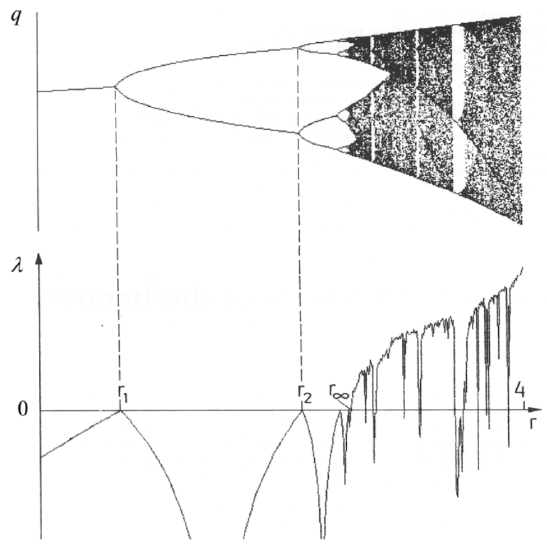
Figure 9.3. The Lyapunov exponent for the logistic map. Adapted, with permission, from the monograph by Schuster and Just (cited below). C Wiley-VCH Verlag \(\mathrm{GmbH}\) & Co. KGaA.
Note that at \(r<r_{\infty}, \lambda\) is negative, indicating the sequence’s stability, besides the points \(r_{1}, r_{2}, \ldots\) where \(\lambda\) would become positive if the limit cycle changes (bifurcations) had not brought it back into the negative territory. However, at \(r>r_{\infty}, \lambda\) becomes positive, returning to negative values only in limited intervals of stable limit cycles. It is evident that in numerical experiments (which dominate the studies of deterministic chaos) the Lyapunov exponent may be used as a good measure of the chaos’ depth. \({ }^{8}\)
Despite all the abundance of results published for particular maps, \({ }^{9}\) and several interesting general observations (like the existence of the Feigenbaum bifurcation sequences), to the best of my knowledge, nobody can yet predict the patterns like those shown in Figure 2 and 3 from just looking at the mapping rule itself, i.e. without carrying out actual numerical experiments. Unfortunately, the understanding of deterministic chaos in other systems is not much better.
\({ }^{1}\) It may be traced back at least to an 1892 paper by the same Jules Henri Poincaré who was already reverently mentioned in Chapter 5. Citing it: "...it may happen that small differences in the initial conditions produce very great ones in the final phenomena. [...] Prediction becomes impossible."
\({ }_{2}\) Its chaotic properties were first discussed in 1976 by Robert May, though the map itself is one of the simple ecological models repeatedly discussed much earlier, and may be traced back at least to the 1838 work by Pierre François Verhulst.
\({ }^{3}\) Since the maximum value of the function \(f(q)\), achieved at \(q=1 / 2\), equals \(r / 4\), the mapping may be limited to segment \(x=[0,1]\), if the parameter \(r\) is between 0 and 4. Since all interesting properties of the map, including chaos, may be found within these limits, I will discuss only this range of \(r\).
\({ }^{4}\) The reader should remember that just as the usual ("nature") experiments, numerical experiments also have limited accuracy, due to unavoidable rounding errors.
\({ }^{5}\) The geometry of these regions is essentially fractal, i.e. has a dimensionality intermediate between 0 (which any final set of geometric points would have) and 1 (pertinent to a 1D continuum). An extensive discussion of fractal geometries and their relation to the deterministic chaos may be found, e.g., in the book by B. Mandelbrot, The Fractal Geometry of Nature, W. H. Freeman, \(1983 .\)
\({ }^{6}\) This does not mean that chaos’ development is always a monotonic function of \(r\). As Figure 2 shows, within certain intervals of this parameter, the chaotic behavior suddenly disappears, being replaced, typically, with a fewpoint limit cycle, just to resume on the other side of the interval. Sometimes (but not always!) the "route to chaos" on the borders of these intervals follows the same Feigenbaum sequence of period-doubling bifurcations.
\({ }^{7}\) After Alexandr Mikhailovich Lyapunov (1857-1918), famous for his studies of the stability of dynamic systems.
\({ }^{8} N\)-dimensional maps that relate \(N\)-dimensional vectors rather than scalars, may be characterized by \(N\) Lyapunov exponents rather than one. For chaotic behavior, it is sufficient for just one of them to become positive. For such systems, another measure of chaos, the Kolmogorov entropy, may be more relevant. This measure, and its relation with the Lyapunov exponents, are discussed, for example, in SM Sec. \(2.2\).
\({ }^{9}\) See, e.g., Chapters 2-4 in H. Schuster and W. Just, Deterministic Chaos, \(4^{\text {th }}\) ed., Wiley-VCH, 2005, or Chapters 8-9 in J. Thompson and H. Stewart, Nonlinear Dynamics and Chaos, \(2^{\text {nd }}\) ed., Wiley, 2002 .