10.3: The Hamilton Principle

Now let me show that the Lagrange equations of motion, that were derived in Sec. \(2.1\) from the Newton laws, may be also obtained from the so-called Hamilton principle, \({ }^{16}\) namely the condition of a minimum (or rather an extremum) of the following integral called action: \[S \equiv \int_{t_{\text {ini }}}^{t_{\text {fin }}} L d t,\] where \(t_{\text {ini }}\) and \(t_{\text {fin }}\) are, respectively, the initial and final moments of time, at which all generalized coordinates and velocities are considered fixed (not varied) - see Figure \(2 .\)

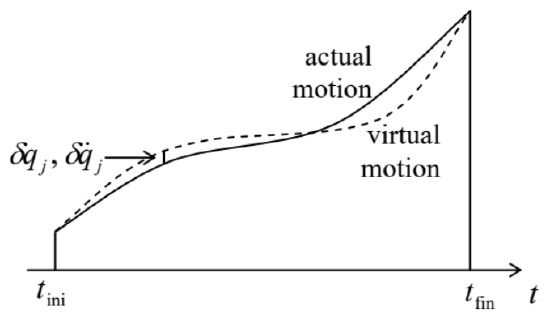Figure 10.2. Deriving the Hamilton principle.

The proof of that statement (in the realm of classical mechanics) is rather simple. Considering, similarly to Sec. 2.1, a possible virtual variation of the motion, described by infinitesimal deviations \(\left\{\delta q_{j}(t), \delta \dot{q}_{j}(t)\right\}\) from the real motion, the necessary condition for \(S\) to be minimal is \[\delta S \equiv \int_{t_{\text {ini }}}^{t_{\text {fin }}} \delta L d t=0,\] where \(\delta S\) and \(\delta L\) are the variations of the action and the Lagrange function, corresponding to the set \(\left\{\delta q_{j}(t), \delta \ddot{q}_{j}(t)\right\}\). As has been already discussed in Sec. 2.1, we can use the operation of variation just as the usual differentiation (but at a fixed time, see Figure 2), swapping these two operations if needed see Figure \(2.3\) and its discussion. Thus, we may write \[\delta L=\sum_{j}\left(\frac{\partial L}{\partial q_{j}} \delta q_{j}+\frac{\partial L}{\partial \dot{q}_{j}} \delta \ddot{q}_{j}\right)=\sum_{j} \frac{\partial L}{\partial q_{j}} \delta q_{j}+\sum_{j} \frac{\partial L}{\partial \dot{q}_{j}} \frac{d}{d t} \delta q_{j} .\] After plugging the last expression into Eq. (48), we can integrate the second term by parts: \[\begin{aligned} \delta S &=\int_{t_{\mathrm{ini}}}^{t_{\mathrm{fin}}} \sum_{j} \frac{\partial L}{\partial q_{j}} \delta q_{j} d t+\sum_{j} \int_{t_{\mathrm{ini}}}^{t_{\mathrm{fin}}} \frac{\partial L}{\partial \dot{q}_{j}} \frac{d}{d t} \delta q_{j} d t \\ &=\int_{t_{\mathrm{ini}}}^{t_{\mathrm{fin}}} \sum_{j} \frac{\partial L}{\partial q_{j}} \delta q_{j} d t+\sum_{j}\left[\frac{\partial L}{\partial \dot{q}_{j}} \delta q_{j}\right]_{t_{\mathrm{ini}}}^{t_{\mathrm{fin}}}-\sum_{j} \int_{t_{\mathrm{ini}}}^{t_{\mathrm{fin}}} \delta q_{j} d\left(\frac{\partial L}{\partial \dot{q}_{j}}\right)=0 \end{aligned}\] Since the generalized coordinates in the initial and final points are considered fixed (not affected by the variation), all \(\delta q_{j}\left(t_{\mathrm{ini}}\right)\) and \(\delta q_{j}\left(t_{\mathrm{fin}}\right)\) vanish, so that the second term in the last form of Eq. (50) vanishes as well. Now multiplying and dividing the last term of that expression by \(d t\), we finally get \[\delta S=\int_{t_{\mathrm{ini}}}^{t_{\mathrm{fin}}} \sum_{j} \frac{\partial L}{\partial q_{j}} \delta q_{j} d t-\sum_{j} \int_{t_{\mathrm{ini}}}^{t_{\mathrm{fin}}} \delta q_{j} \frac{d}{d t}\left(\frac{\partial L}{\partial \dot{q}_{j}}\right) d t=-\int_{t_{\mathrm{ini}}}^{t_{\mathrm{fin}}} \sum_{j}\left[\frac{d}{d t}\left(\frac{\partial L}{\partial \dot{q}_{j}}\right)-\frac{\partial L}{\partial q_{j}}\right] \delta q_{j} d t=0\] This relation should hold for an arbitrary set of functions \(\delta q_{j}(t)\), and for any time interval, and this is only possible if the expressions in the square brackets equal zero for all \(j\), giving us the set of the Lagrange equations (2.19). So, the Hamilton principle indeed gives the Lagrange equations of motion.

It is fascinating to see how does the Hamilton principle work for particular cases. As a very simple example, let us consider the usual 1D linear oscillator, with the Lagrangian function used so many times before in this course: \[L=\frac{m}{2} \dot{q}^{2}-\frac{m \omega_{0}^{2}}{2} q^{2} .\] As we know very well, the Lagrange equations of motion for this \(L\) are exactly satisfied by any sinusoidal function with the frequency \(\omega_{0}\), in particular by a symmetric function of time \[q_{\mathrm{e}}(t)=A \cos \omega_{0} t, \quad \text { so that } \dot{q}_{\mathrm{e}}(t)=-A \omega_{0} \sin \omega_{0} t .\] On a limited time interval, say \(0 \leq \omega_{0} t \leq+\pi / 2\), this function is rather smooth and may be well approximated by another simple, reasonably selected functions of time, for example \[q_{\mathrm{a}}(t)=A\left(1-\lambda t^{2}\right), \quad \text { so that } \dot{q}_{\mathrm{a}}(t)=-2 A \lambda t,\] provided that the parameter \(\lambda\) is also selected in a reasonable way. Let us take \(\lambda=\left(\pi / 2 \omega_{0}\right)^{2}\), so that the approximate function \(q_{\mathrm{a}}(t)\) coincides with the exact function \(q_{\mathrm{e}}(t)\) at both ends of our time interval (Figure 3): \[q_{\mathrm{a}}\left(t_{\mathrm{ini}}\right)=q_{\mathrm{e}}\left(t_{\mathrm{ini}}\right)=A, \quad q_{\mathrm{a}}\left(t_{\mathrm{fin}}\right)=q_{\mathrm{e}}\left(t_{\mathrm{fin}}\right)=0, \quad \text { where } t_{\mathrm{ini}} \equiv 0, \quad t_{\mathrm{fin}} \equiv \frac{\pi}{2 \omega_{0}},\] and check which of them the Hamilton principle "prefers", i.e. which function gives the least action.

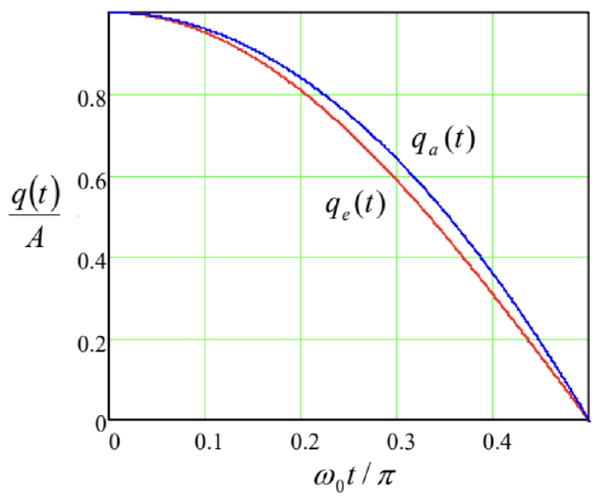
Figure 10.3. Plots of the functions \(q(t)\) given by Eqs. (53) and (54).

An elementary calculation of the action (47), corresponding to these two functions, yields \[S_{\mathrm{e}}=\left(\frac{\pi}{8}-\frac{\pi}{8}\right) m \omega_{0} A^{2}=0, \quad S_{\mathrm{a}}=\left(\frac{4}{3 \pi}-\frac{2 \pi}{15}\right) m \omega_{0} A^{2} \approx(0.4244-0.4189) m \omega_{0} A^{2}>0,\] with the first terms in all the parentheses coming from the time integrals of the kinetic energy, and the second terms, from those of the potential energy.

This result shows, first, that the exact function of time, for which these two contributions exactly cancel, \({ }^{17}\) is indeed "preferable" for minimizing the action. Second, for the approximate function, the two contributions to the action are rather close to the exact ones, and hence almost cancel each other, signaling that this approximation is very reasonable. It is evident that in some cases when the exact analytical solution of the equations of motion cannot be found, the minimization of \(S\) by adjusting one or more free parameters, incorporated into a guessed "trial" function, may be used to find a reasonable approximation for the actual law of motion. 18It is also very useful to make the notion of action \(S\), defined by Eq. (47), more transparent by calculating it for the simple case of a single particle moving in a potential field that conserves its energy \(E=T+U\). In this case, the Lagrangian function \(L=T-U\) may be represented as \[L=T-U=2 T-(T+U)=2 T-E=m v^{2}-E,\] with a time-independent \(E\), so that \[S=\int L d t=\int m v^{2} d t-E t+\text { const. }\] Representing the expression under the remaining integral as \(m \mathbf{v} \cdot \mathbf{v} d t=\mathbf{p} \cdot(d \mathbf{r} / d t) d t=\mathbf{p} \cdot d \mathbf{r}\), we finally get \[S=\int \mathbf{p} \cdot d \mathbf{r}-E t+\text { const }=S_{0}-E t+\text { const },\] where the time-independent integral \[S_{0} \equiv \int \mathbf{p} \cdot d \mathbf{r}\] is frequently called the abbreviated action.

This expression may be used to establish one more important connection between classical and quantum mechanics - now in its Schrödinger picture. Indeed, in the quasiclassical (WKB) approximation of that picture \({ }^{19}\) a particle of fixed energy is described by a de Broglie wave \[\Psi(\mathbf{r}, t) \propto \exp \left\{i\left(\int \mathbf{k} \cdot d \mathbf{r}-\omega t+\text { const }\right)\right\},\] where the wave vector \(\mathbf{k}\) is proportional to the particle’s momentum, and the frequency \(\omega\), to its energy: \[\mathbf{k}=\frac{\mathbf{p}}{\hbar}, \quad \omega=\frac{E}{\hbar} .\] Plugging these expressions into Eq. (61) and comparing the result with Eq. (59), we see that the WKB wavefunction may be represented as \[\Psi \propto \exp \{i S / \hbar\} .\] Hence Hamilton’s principle (48) means that the total phase of the quasiclassical wavefunction should be minimal along the particle’s real trajectory. But this is exactly the so-called eikonal minimum principle well known from the optics (though valid for any other waves as well), where it serves to define the ray paths in the geometric optics limit - similar to the WKB approximation condition. Thus, the ratio \(S / \hbar\) may be considered just as the eikonal, i.e. the total phase accumulation, of the de Broglie waves. \({ }^{20}\)

Now, comparing Eq. (60) with Eq. (39), we see that the action variable \(J\) is just the change of the abbreviated action \(S_{0}\) along a single phase-plane contour (divided by \(2 \pi\) ). This means, in particular, that in the WKB approximation, \(J\) is the number of de Broglie waves along the classical trajectory of a particle, i.e. an integer value of the corresponding quantum number. If the system’s parameters are changed slowly, the quantum number has to stay integer, and hence \(J\) cannot change, giving a quantummechanical interpretation of the adiabatic invariance. This is really fascinating: a fact of classical mechanics may be "derived" (or at least understood) more easily from the quantum mechanics’ standpoint. \({ }^{21}\)

---

\({ }^{16}\) It is also called the "principle of least action", or the "principle of stationary action". (These names may be fairer in the context of a long history of the development of the principle, starting from its simpler particular forms, which includes the names of P. de Fermat, P. Maupertuis, L. Euler, and J.-L. Lagrange.)

\({ }^{17}\) Such cancellation, i.e. the equality \(S=0\), is of course not the general requirement; it is specific only for this particular example.

\({ }^{18}\) This is essentially a classical analog of the variational method of quantum mechanics - see, e.g., QM Sec. \(2.9 .\)

\({ }^{19}\) See, e.g., QM Sec. 3.1.

\({ }^{20}\) Indeed, Eq. (63) was the starting point for R. Feynman’s development of his path-integral formulation of quantum mechanics - see, e.g., QM Sec. 5.3.

\({ }^{21}\) As a reminder, we have run into a similarly pleasant surprise at our discussion of the non-degenerate parametric excitation in Sec. \(6.7\).

\({ }^{22}\) See, e.g., Chapters 6-9 in I. C. Percival and D. Richards, Introduction to Dynamics, Cambridge U. Press, \(1983 .\)