1.3: Not So Tight

In fact, there are hidden approximations in the above analysis—for one thing, we’ve assumed that the length of string between \(\begin{equation}x \text { and } x+d x \text { is } d x\end{equation}\), but it’s really ds, where the distance parameter s is measured along the string. Second, we took the tension to be nonvarying. That’s a pretty good approximation for a string that’s almost horizontal, but think about a string a meter long hanging between two points 5 cm apart, and it becomes obvious that both these approximations are only good for a near-horizontal string.

Obviously, with the string nearly vertical, the tension is balancing the weight of string below it, and must be close to zero at the bottom, increasing approximately linearly with height. Not to mention, it’s clear that this is no parabola, the two sides are very close to parallel near the top. The constant \(\begin{equation}T\end{equation}\) approximation is evidently no good—but Whewell solved this problem exactly, back in the 1830’s.

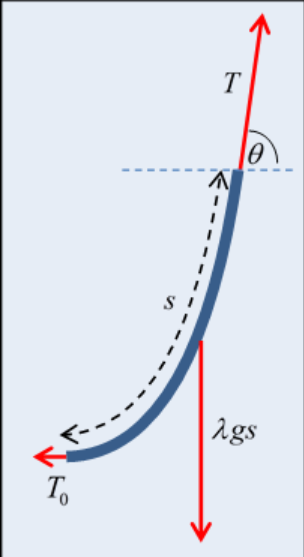
What he did was to work with the static equilibrium equation for a finite length of string, one end at the bottom.

If the tension at the bottom is \(\begin{equation}T_{0}\end{equation}\) and at a distance s away, measured along the string, the tension is \(T\), and the string’s angle to the horizontal there is \(\theta\) (see diagram), then the equilibrium balance of force components is

\begin{equation}T \cos \theta=T_{0}, \quad T \sin \theta=\lambda g s\end{equation}

from which the string slope

\begin{equation}\tan \theta=\frac{\lambda g}{T_{0}} s=\frac{s}{a}\end{equation}

where we have introduced the constant \(\begin{equation}a=T_{0} / \lambda g\end{equation}\), which sets the length scale of the problem.

So we now have an equation for the catenary, \(\theta\) in terms of s, distance along the string. What we want, though is an equation for vertical position \(y\) in terms of horizontal position \(x\), the function \(\begin{equation}y(x)\end{equation}\) for the chain.

Now we’ve shown the slope is

\begin{equation}d y / d x=\tan \theta=s / a\end{equation}

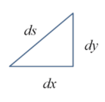
and the infinitesimals are related by \(\begin{equation}d s^{2}=d x^{2}+d y^{2}\end{equation}\), so putting these equations together

\begin{equation}\left(\frac{s}{a}\right)^{2}=\left(\frac{d y}{d x}\right)^{2}=\left(\frac{d s}{d x}\right)^{2}-1\end{equation}

that is,

\begin{equation}\left(\frac{d s}{d x}\right)^{2}=1+\left(\frac{s}{a}\right)^{2}=\frac{a^{2}+s^{2}}{a^{2}}\end{equation}

Taking the square root and rearranging

\begin{equation}\frac{d s}{\sqrt{a^{2}+s^{2}}}=\frac{d x}{a}\end{equation}

which can be integrated immediately with the substitution

\begin{equation}s=a \sinh \xi, \quad d s=a \cosh \xi d \xi\end{equation}

to give just

\begin{equation}d \xi=d x / a\end{equation}

which integrates trivially to \(\begin{equation}\xi=(x / a)+b, \text { with } b\end{equation}\) a constant of integration, or

\begin{equation}s=a \sinh \xi=a \sinh (x / a)\end{equation}

choosing the origin \(\begin{equation}x=0 \text { at } s=0, \text { which makes } b=0\end{equation}\)

But of course what we want is the curve shape \(\begin{equation}y(x), \text { not } s(x)\end{equation}\). We need to eliminate \(s\) in the favor of \(y\). That is, we need to write \(y\) as a function of \(s\), then substitute \(\begin{equation}s=a \sinh (x / a)\end{equation}\)

Recall one of our first equations was for the slope \(\begin{equation}d y / d x=s / a\end{equation}\), and putting that together with \(\begin{equation}s=a \sinh (x / a)\end{equation}\) gives

\begin{equation}a d y=s d x=a \sinh (x / a) d x\end{equation}

integrating to

\begin{equation}y=a \cosh (x / a)\end{equation}

This is the desired equation for the catenary curve \(\begin{equation}y(x)\end{equation}\)

We’ve dropped the possible constant of integration, which is just the vertical positioning of the origin.

Question: is this the same as the curve of the chain in a suspension bridge?

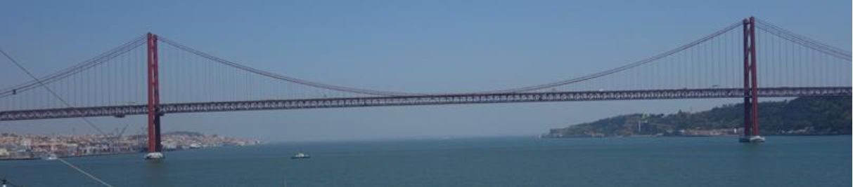
(Notice the vertical ropes are uniformly spaced horizontally.)