2.14: Newton's Law of Gravitation

Gravitation plays a fundamental role in classical mechanics as well as being an important example of a conservative central $\big ( \frac{1}{r} \big ) ^2$ force. Although you may not be familiar with the following presentation addressing the gravitational field $\mathbf{g}$, it is assumed that you have met the identical discussion when addressing the electric field $\mathbf{E}$ in electrostatics. The only difference is that mass $m$ replaces charge $e$ and gravitational field $\mathbf{g}$ replaces the electric field $\mathbf{E}$. Thus this chapter is designed to be a review of the concepts that can be used for study of any conservative inverse-square law central fields.

In 1666 Newton formulated the Theory of Gravitation which he eventually published in the Principia in 1687. Newton’s Law of Gravitation states that each mass particle attracts every other particle in the universe with a force that varies directly as the product of the mass and inversely as the square of the distance between them. That is, the force on a gravitational point mass $m_G$ produced by a mass $M_G$

$$\label{eq:2.143} \mathbf{F}_m = -G \frac{m_G M_G}{r^2} \hat{\mathbf{r}}$$

where $\hat{\mathbf{r}}$ is the unit vector pointing from the gravitational mass $M_G$ to the gravitational mass $m_g$ as shown in Figure $\PageIndex{1}$. Note that the force is attractive, that is, it points toward the other mass. This is in contrast to the repulsive electrostatic force between two similar charges. Newton’s law was verified by Cavendish using a torsion balance. The experimental value of $G = (6.6726 \pm 0.0008 \times 10^{-11} \ N \times m^2 / kg^2$

The gravitational force between point particles can be extended to finite-sized bodies using the fact that the gravitational force field satisfies the superposition principle, that is, the net force is the vector sum of the individual forces between the component point particles. Thus the force summed over the mass distribution is

$$\label{eq:2.144} \mathbf{F} ( \mathbf{r} )_m = - G m_G \sum_{i=1}^n \frac{m_{G_i}}{r_i^2} \hat{\mathbf{r}}_i$$

where $\mathbf{r}_i$ is the vector from the gravitational mass $m_{G_i}$ to the gravitational mass $m_G$ at the position $\mathbf{r}$.

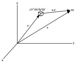
For a continuous gravitational mass distribution $\rho_G ( \mathbf{r^\prime} )$, the net force on the gravitational mass $m_G$ at the location $\mathbf{r}$ can be written as

$$\label{eq:2.145} \mathbf{F}_m ( \mathbf{R} ) = -G m_G \int_v \frac{ \rho_G ( \mathbf{r^\prime} )\big ( \mathbf{\hat{r} - \hat{r^\prime} } \big ) }{ ( \mathbf{ \bar{r} - \bar{r^\prime} } ) ^2 } dv^\prime$$

where $dv^\prime$ is the volume element at the point $\mathbf{r^\prime }$ as illustrated in Figure $\PageIndex{1}$.

Figure $\PageIndex{1}$: Gravitational force on mass m due to an infinitessimal volume element of the mass density distribution.

Gravitational and inertial mass

Newton's Laws use the concept of inertial mass $m_I \equiv m$ in relating the force $\mathbf{F}$ to acceleration $\mathbf{a}$

$$\label{eq:2.146} \mathbf{F} = m_I \mathbf{a}$$

and momentum $\mathbf{p}$ to velocity $\mathbf{v}$

$$\label{eq:2.147} \mathbf{p} = m_I \mathbf{v}$$

That is, inertial mass is the constant of proportionality relating the acceleration to the applied force.

The concept of gravitational mass $m_G$ is the constant of proportionality between the gravitational force and the amount of matter. That is, on the surface of the earth, the gravitational force is assumed to be

$$\label{eq:2.148} \mathbf{F}_G = m_G \bigg [ -G \sum_{i=1}^n \frac{m_{G_i}}{r_i^2} \hat{\mathbf{r}}_i \bigg ] = m_G \mathbf{g}$$

where $\mathbf{g}$ is the gravitational field which is a position-dependent force per unit gravitational mass pointing towards the center of the Earth. The gravitational mass is measured when an object is weighed.

Newton’s Law of Gravitation leads to the relation for the gravitational field $\mathbf{g ( r ) }$ at the location $\mathbf{r}$ due to a gravitational mass distribution at the location $\mathbf{r}^\prime$ as given by the integral over the gravitational mass density $\rho_G$

$$\label{eq:2.149} \mathbf{g ( r )} = -G \int_V \frac{ \rho_G ( \mathbf{r}^{\prime} ) \big ( \mathbf{\hat{r} - \hat{r}{^\prime} } \big ) }{ ( \mathbf{ \bar{r} - \bar{r}^{\prime} } ) ^2 } d v^\prime$$

The acceleration of matter in a gravitational field relates the gravitational and inertial masses

$$\label{eq:2.150} \mathbf{F} _G = m_G \mathbf{g} = m_I \mathbf{a}$$

Thus

$$\label{eq:2.151} \mathbf{a} = \frac{m_G}{m_I} \mathbf{g}$$

That is, the acceleration of a body depends on the gravitational strength $g$ and the ratio of the gravitational and inertial masses. It has been shown experimentally that all matter is subject to the same acceleration in vacuum at a given location in a gravitational field. That is, $\frac{m_G }{m_I}$ is a constant common to all materials. Galileo first showed this when he dropped objects from the Tower of Pisa. Modern experiments have shown that this is true to 5 parts in 10¹³.

The exact equivalence of gravitational mass and inertial mass is called the weak principle of equivalence which underlies the General Theory of Relativity as discussed in chapter $17$. It is convenient to use the same unit for the gravitational and inertial masses and thus they both can be written in terms of the common mass symbol $m$.

$$\label{eq:2.152} m_I = m_G = m$$

Therefore the subscripts $G$ and $I$ can be omitted in equations $\ref{eq:2.150}$ and $\ref{eq:2.152}$. Also the local acceleration due to gravity $\mathbf{a}$ can be written as

$$\label{eq:2.153} \mathbf{a = g}$$

The gravitational field $\mathbf{g} \equiv \frac{\mathbf{F}}{m}$ has units of N/kg in the MKS system while the acceleration $\mathbf{a}$ has units $m/s^2$.

Gravitational potential energy $U$

Chapter $2.10.2$ showed that a conservative field can be expressed in terms of the concept of a potential energy $U( \mathbf{r})$ which depends on position. The potential energy difference $\Delta U_{a \rightarrow b}$ between two points $\mathbf{r}_a$ and $\mathbf{r}_b$, is the work done moving from $a$ to $b$ against a force $\mathbf{F}$. That is:

$$\label{eq:2.154} \Delta U_{a \rightarrow b} = U( \mathbf{r}_b ) - U( \mathbf{r}_a ) = - \int_{r_a}^{r_b} \mathbf{F} \cdot d\mathbf{l}$$

In general, this line integral depends on the path taken.

Consider the gravitational field produced by the single point mass $m_1$. The work done moving a mass $m_0$ from $r_a$ to $r_b$ in this gravitational field can be calculate along an arbitrary path shown in Figure $\PageIndex{2}$ by assuming Newton's law of gravitation. Then the force on $m_0$ due to point mass $m_1$ is:

$$\label{eq:2.155} \mathbf{F} = - G \frac{m_1 m_0}{r^2} \hat{\mathbf{r}}$$

Figure $\PageIndex{2}$: Work done against a force field moving from a to b.

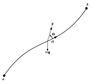
Expressing $d\mathbf{l}$ in spherical coordinates $d\mathbf{l} = dr \mathbf{\hat{r}} + rd\theta \mathbf{\hat{\theta}} + r \sin \theta d \phi \mathbf{\hat{\phi}}$ gives that the path integral $\ref{eq:2.154}$ from $( r_a \theta_a \phi_a )$ to $( r_b \theta_b \phi_b )$ is

$$\label{eq:2.156} \begin{split} \Delta U_{a \rightarrow b} & = & - \int_a^b \mathbf{F} \cdot d\mathbf{l} = \int_a^b \big [ G \frac{m_1m_2}{r^2} ( \mathbf{\hat{r} \cdot \widehat{r}} dr + \mathbf{\hat{r}} \cdot \mathbf{\hat{\theta}} d \theta + r \sin \theta \mathbf{\hat{r}} \cdot \hat{\mathbf{\phi}} d \phi ) \big ] = G \int_a^b \frac{m_1m_0}{r^2} \widehat{\mathbf{r}} \cdot \widehat{\mathbf{r}} dr \\ & = & -Gm_1m_0 \Big [ \frac{1}{r_b} - \frac{1}{r_a} \Big ] \end{split}$$

since the scalar product of the unit vectors $\mathbf{ \widehat{r} \cdot \widehat{r}} = 1$. Note that the second two terms also cancel since $\mathbf{ \widehat{r} \cdot \hat{\theta}} = \mathbf{\hat{r} \cdot \hat{\phi}} = 0$ since the unit vectors are mutually orthogonal. Thus the line integral just depends only on the starting and ending radii and is independent of the angular coordinates or the detailed path taken between $( r_a \theta_a \phi_a )$ and $( r_b \theta_b \phi_b )$.

Consider the Principle of Superposition for a gravitational field produced by a set of n point masses. The line integral then can be written as

$$\label{eq:2.157} \Delta U_{a \rightarrow b }^{net} = -\int_{r_a}^{r_b} \mathbf{F}_{net} \cdot d \mathbf{l} = - \sum_{i=1}^n \int_{r_a}^{r_b} \mathbf{F}_i \cdot d \mathbf{l} = \sum_{i=1}^n \Delta U _{a \rightarrow b}^i$$

Thus the net potential energy difference is the sum of the contributions from each point mass producing the gravitational force field. Since each component is conservative, then the total potential energy difference also must be conservative. For a conservative force, this line integral is independent of the path taken, it depends only on the starting and ending positions, $\mathbf{r}_a$ and $\mathbf{r}_b$. That is, the potential energy is a local function dependent only on position. The usefulness of gravitational potential energy is that, since the gravitational force is a conservative force, it is possible to solve many problems in classical mechanics using the fact that the sum of the kinetic energy and potential energy is a constant. Note that the gravitational field is conservative, since the potential energy difference $\Delta_{a \rightarrow b}^{net}$ is independent of the path taken. It is conservative because the force is radial and time independent, it is not due to the $\frac{1}{r^2}$ dependence of the field.

Gravitational potential $\phi$

Using $\mathbf{F} = m_0\mathbf{g}$ gives that the change in potential energy due to moving a mass $m_0$ from $a$ to $b$ in a gravitational field $\mathbf{g}$ is:

$$\label{eq:2.158} \Delta U_{a \rightarrow b}^{net} = - m_0 \int_{r_a}^{r_b} \mathbf{g}_{net}\cdot d\mathbf{l}$$

Note that the probe mass $m_0$ factors out from the integral. It is convenient to define a new quantity called gravitational potential $\phi$ where

$$\label{eq:2.159} \Delta_{a \rightarrow b}^{net} = \frac{\Delta U_{a \rightarrow b}^{net}}{m_0} = -\int_{r_a}^{r_b} \mathbf{g}_{net} \cdot d \mathbf{l}$$

That is; gravitational potential difference is the work that must be done, per unit mass, to move from $a$ to $b$ with no change in kinetic energy. Be careful not to confuse the gravitational potential energy difference $\Delta U _{a \rightarrow b }$ and gravitational potential difference $\Delta \phi_{a \rightarrow b}$, that is, $\Delta U$ has units of energy, Joules_, while $\Delta \phi$ has units of Joules/Kg.

The gravitational potential is a property of the gravitational force field; it is given as minus the line integral of the gravitational field from $a$ to $b$. The change in gravitational potential energy for moving a mass $m_0$ from $a$ to $b$ is given in terms of gravitational potential by:

$$\label{eq:2.160} \Delta U _{a \rightarrow b} ^{net} = m_0 \Delta \phi_{a \rightarrow b }^{net}$$

Superposition and potential

Previously it was shown that the gravitational force is conservative for the superposition of many masses.

To recap, if the gravitational field

$$\label{eq:2.161} \mathbf{g}_{net} = \mathbf{g_1 + g_2 + g_3 }$$

then

$$\label{eq: 2.162} \phi_{a \rightarrow b}^{net} = - \int_{r_a}^{r_b} \mathbf{g}_{net} \cdot d \mathbf{l} = - \int_{r_a}^{r_b} \mathbf{g}_1 \cdot d \mathbf{l} - \int_{r_a}^{r_b} \mathbf{g}_2 \cdot d \mathbf{l} - \int_{r_a}^{r_b} \mathbf{g}_3 \cdot d \mathbf{l} = \sum_i^n \phi_{a\rightarrow b} ^{i}$$

Thus gravitational potential is a simple additive scalar field because the Principle of Superposition applies. The gravitational potential, between two points differing by $h$ in height, is $gh$. Clearly, the greater $g$ or $h$, the greater the energy released by the gravitational field when dropping a body through the height $h$. The unit of gravitational potential is the $\frac{Joule}{Kg}$

Potential theory

The gravitational force and electrostatic force both obey the inverse square law, for which the field and corresponding potential are related by:

$$\label{eq:2.163} \Delta \phi_{a \rightarrow b } = -\int_{r_a}^{r_b} \mathbf{g} \cdot d \mathbf{l}$$

for an arbitrary infinitessimal element distance $d\mathbf{l}$ the change in electric potential $d \phi$ is

$$\label{eq:2.164} d \phi= - \mathbf{g} \cdot d \mathbf{l}$$

Using cartesian coordinates both $\mathbf{g}$ and $d \mathbf{l}$ can be written as

$$\label{eq:2.165} \mathbf{g} = \mathbf{\widehat{i}}g_x + \mathbf{\widehat{j}}g_y + \mathbf{\widehat{k}}g_z \hspace{6cm} d \mathbf{l} = \mathbf{\widehat{i}}dx + \mathbf{\widehat{j}}dy + \mathbf{\widehat{k}}dz$$

Taking the scalar product gives:

$$\label{eq:2.166} d \phi = - \mathbf{g} \cdot d \mathbf{l} = - g_x dx - g_y dy - g_z dz$$

Differential calculus expresses the change in potential $d \phi$ in terms of partial derivatives by:

$$\label{eq:2.167} d \phi = \frac{\partial \phi}{\partial x} dx + \frac{\partial \phi}{\partial y} dy + \frac{\partial \phi}{\partial z} dz$$

By association, $\ref{eq:2.166}$ and $\ref{eq:2.167}$ imply that

$$\label{eq:2.168} \begin{align} g_x = - \frac{\partial \phi}{\partial x} & \hspace{2cm} g_y = - \frac{\partial \phi}{\partial y} & g_z = - \frac{\partial \phi}{\partial z} \end{align}$$

Thus on each axis, the gravitational field can be written as minus the gradient of the gravitational potential. In three dimensions, the gravitational field is minus the total gradient of potential and the gradient of the scalar function $\phi$ can be written as:

$$\label{eq:2.169} \mathbf{g} = - \mathbf{\nabla} \phi$$

In cartesian coordinates this equals

$$\label{eq:2.170}\mathbf{g} = - \Big [ \mathbf{\widehat{i}}\frac{\partial \phi} {\partial x} + \mathbf{\widehat{j}}\frac{\partial \phi}{\partial y} + \mathbf{\widehat{k}}\frac{\partial \phi}{\partial z} \Big ]$$

Thus the gravitational field is just the gradient of the gravitational potential, which always is perpendicular to the equipotentials. Skiers are familiar with the concept of gravitational equipotentials and the fact that the line of steepest descent, and thus maximum acceleration, is perpendicular to gravitational equipotentials of constant height. The advantage of using potential theory for inverse-square law forces is that scalar potentials replace the more complicated vector forces, which greatly simplifies calculation. Potential theory plays a crucial role for handling both gravitational and electrostatic forces.

Curl of gravitational field

It has been shown that the gravitational field is conservative, that is $\Delta U _ {a \rightarrow b}$ is independent of the path taken between $a$ and $b$ Therefore, Equation $\ref{eq:2.159}$ gives that the gravitational potential is independent of the path taken between two points $a$ and $b$. Consider two possible paths between $a$ and $b$ as shown in Figure $\PageIndex{3}$. The line integral from $a$ to $b$ via route 1 is equal and opposite to the line integral back from $b$ to $a$ via route 2 if the gravitational field is conservative as shown earlier.

Figure $\PageIndex{3}$: Circulation of the gravitational field.

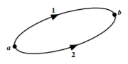
A better way of expressing this is that the line integral of the gravitational field is zero around any closed path. Thus the line integral between $a$ and $b$, via path 1, and returning back to $a$, via path 2, are equal and opposite. That is, the net line integral for a closed loop is zero.

$$\label{eq:2.171} \oint \mathbf{g}_{net} \cdot d \mathbf{l} = 0$$

which is a measure of the circulation of the gravitational field. The fact that the circulation equals zero corresponds to the statement that the gravitational field is radial for a point mass.

Stokes Theorem, discussed in appendix $19.8.3$, states that

$$\label{eq:2.172} \oint_C \mathbf{F} \cdot d \mathbf{l} = \int_{\substack{Area \\ bounded \\ by \\ C }} ( \mathbf{\nabla} \times \mathbf{F} ) \cdot d \mathbf{S}$$

Thus the zero circulation of the gravitational field can be rewritten as

$$\label{eq:2.173} \oint_C \mathbf{g} \cdot d \mathbf{l} = \int_{\substack{Area \\ bounded \\ by \\ C }} ( \mathbf{\nabla} \times \mathbf{g} ) \cdot d \mathbf{S} = 0$$

Since this is independent of the shape of the perimeter $C$, therefore

$$\label{eq:2.174} \mathbf{\nabla} \times \mathbf{g} = 0$$

That is, the gravitational field is a curl-free field.

A property of any curl-free field is that it can be expressed as the gradient of a scalar potential $\phi$ since

$$\label{eq:2.175} \nabla \times \nabla \phi = 0$$

Therefore, the curl-free gravitational field can be related to a scalar potential $\phi$ as

$$\label{eq:2.176} \mathbf{g} = - \mathbf{ \nabla} \phi$$

Thus $\phi$ is consistent with the above definition of gravitational potential $\phi$ in that the scalar product

$$\label{eq:2.177} \Delta \phi_{a \rightarrow b} = - \int_a^b \mathbf{g}_{net} \cdot d \mathbf{l} = \int_a^b ( \mathbf{\nabla} \phi ) \cdot d \mathbf{l} = \int_A^b \sum_i \frac{\partial \phi}{\partial x_i}dx_i = \int_a^b d \phi$$

An identical relation between the electric field and electric potential applies for the inverse-square law electrostatic field.

Reference potentials

Note that only differences in potential energy, $U$, and gravitational potential, $\phi$, are meaningful, the absolute values depend on some arbitrarily chosen reference. However, often it is useful to measure gravitational potential with respect to a particular arbitrarily chosen reference point $\phi_a$ such as to sea level. Aircraft pilots are required to set their altimeters to read with respect to sea level rather than their departure airport. This ensures that aircraft leaving from say both Rochester, $559^\prime$ $msl$ and Denver $5000^\prime$ $msl$, have their altimeters set to a common reference to ensure that they do not collide. The gravitational force is the gradient of the gravitational field which only depends on differences in potential, and thus is independent of any constant reference.

Gravitational potential due to continuous distributions of charge

Suppose mass is distributed over a volume $v$ with a density $\rho$ at any point within the volume. the gravitational potential at any field point $p$ due to an element of mass $dm = \rho v$ at the point $p^\prime$ is given by:

$$\label{eq:2.178} \Delta \phi_{\infty \rightarrow p} = -G \int_v \frac{ \rho ( p^\prime ) dv^\prime }{r_{p^\prime p } }$$

This integral is over a scalar quantity. Since gravitational potential $\phi$ is a scalar quantity, it is easier to compute than is the vector gravitational field $\mathbf{g}$. If the scalar potential field is known, then the gravitational field is derived by taking the gradient of the gravitational potential.

Gauss's Law for Gravitation

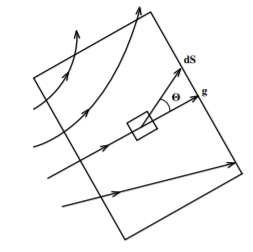
The flux $\Phi$ of the gravitational field $\mathbf{g}$ through a surface $S$, as shown in Figure $\PageIndex{4}$ is defined as

$$\label{eq:2.179} \Phi \equiv \int_S \mathbf{g} \cdot d \mathbf{S}$$

Note that there are two possible perpendicular directions that could be chosen for the surface vector $d \mathbf{S}$. Using Newton’s law of gravitation for a point mass $m$ the flux through the surface $S$ is

$$\label{eq:2.180} \Phi = - Gm \int_S \frac{\widehat{\mathbf{r}} \cdot d \mathbf{S}}{r^2}$$

Note that the solid angle subtended by the surface $dS$ at an angle $\theta$ to the normal from the point mass is given by

$$\label{eq:2.181} d \Omega = \frac{ \cos \theta dS}{r^2} = \frac{\widehat{\mathbf{r}} \cdot d \mathbf{S}}{r^2}$$

Thus the net gravitational flux equals

$$\label{eq:2.182} \Phi = - Gm \int_S d \Omega$$

Figure $\PageIndex{4}$: Flux of the gravitational field through an infinitessimal surface element dS.

Consider a closed surface where the direction of the surface vector $d \mathbf{S}$ is defined as outwards. The net flux out of this closed surface is given by

$$\label{eq:2.183} \Phi = - Gm \oint_S \frac{\widehat{\mathbf{r}} \cdot d \mathbf{S}}{r^2} = - Gm \oint_S d \Omega = - Gm 4 \pi$$

This is independent of where the point mass lies within the closed surface or on the shape of the closed surface. Note that the solid angle subtended is zero if the point mass lies outside the closed surface. Thus the flux is as given by Equation $\ref{eq:2.183}$ if the mass is enclosed by the closed surface, while it is zero if the mass is outside of the closed surface.

Since the flux for a point mass is independent of the location of the mass within the volume enclosed by the closed surface, and using the principle of superposition for the gravitational field, then for n enclosed point masses the net flux is

$$\label{eq:2.184} \Phi \equiv \int_S \mathbf{G} \cdot d \mathbf{S} = - 4 \pi G \sum_i^n m_i$$

This can be extended to continuous mass distributions, with local mass density $\rho$, giving that the net flux

$$\label{eq:2.185} \Phi \equiv \int_S \mathbf{g} \cdot d \mathbf{S} = -4 \pi G \int_{\substack{enclosed \\ volume}} \rho dv$$

Gauss's Divergence Theorem was given in appendix $19.8.2$ as

$$\label{eq:2.186} \Phi = \oint_S \mathbf{F} \cdot d \mathbf{S} = \int_{\substack{enclosed \\ volume}} \mathbf{\nabla} \cdot \mathbf{F} dv$$

Applying the Divergence Theorem to Gauss's law gives that

$$\nonumber \Phi = \oint_s \mathbf{g} \cdot d \mathbf{S} = \int_{\substack{enclosed \\ volume}} \mathbf{\nabla} \cdot \mathbf{g} dv = - 4 \pi G \int_{\substack{enclosed \\ volume}} \rho dv$$

or

$$\label{eq:2.187} \int_{\substack{enclosed \\ volume}} [ \mathbf{\nabla} \cdot \mathbf{g} + 4 \pi G \rho ] dv = 0$$

This is true independent of the shape of the surface, thus the divergence of the gravitational field

$$\label{eq:2.188} \mathbf{\nabla} \cdot \mathbf{g} = -4 \pi G \rho$$

This is a statement that the gravitational field of a point mass has a $\frac{1}{r^2}$ dependence.

Using the fact that the gravitational field is conservative, this can be expressed as the gradient of the gravitational potential $\phi$,

$$\label{eq:2.189} \mathbf{g} = - \mathbf{\nabla} \phi$$

and Gauss’s law, then becomes

$$\label{eq:2.190} \mathbf{\nabla} \cdot \mathbf{\nabla} \phi = 4 \pi G \rho$$

which also can be written as Poisson’s equation

$$\label{eq:2.191} \nabla^2 \phi = 4 \pi G \rho$$

Knowing the mass distribution $\rho$ allows determination of the potential by solving Poisson’s equation. A special case that often is encountered is when the mass distribution is zero in a given region. Then the potential for this region can be determined by solving Laplace’s equation with known boundary conditions.

$$\label{eq:2.192} \nabla^2 \phi = 0$$

For example, Laplace’s equation applies in the free space between the masses. It is used extensively in electrostatics to compute the electric potential between charged conductors which themselves are equipotentials.

Condensed forms of Newton's Law of Gravitation

The above discussion has resulted in several alternative expressions of Newton’s Law of Gravitation that will be summarized here. The most direct statement of Newton’s law is

$$\label{eq:2.193} \mathbf{g ( r ) } = -G \int_V \frac{\rho ( \mathbf{r}^\prime ) \Big ( \mathbf{ \widehat{r} - \widehat{r}} \Big ) }{ ( \mathbf{r} - \mathbf{r}^\prime ) ^2} dv^\prime$$

An elegant way to express Newton’s Law of Gravitation is in terms of the flux and circulation of the gravitational field. That is

Flux:

$$\label{eq:2.194} \Phi \equiv \int_S \mathbf{g} \cdot d \mathbf{S} = - 4\pi G \int_{\substack{enclosed \\ volume}} \rho dv$$

Circulation:

$$\label{eq:2.195} \oint \mathbf{g}_{net} \cdot d \mathbf{l} = 0$$

The flux and circulation are better expressed in terms of the vector differential concepts of divergence and curl.

Divergence:

$$\label{eq:2.196} \mathbf{\nabla} \cdot \mathbf{g} = -4 \pi G \rho$$

Curl:

$$\label{eq:2.197} \mathbf{\nabla} \times \mathbf{g} = 0$$

Remember that the flux and divergence of the gravitational field are statements that the field between point masses has a $\frac{1}{r^2}$ dependence. The circulation and curl are statements that the field between point masses is radial.

Because the gravitational field is conservative it is possible to use the concept of the scalar potential field $\phi$. This concept is especially useful for solving some problems since the gravitational potential can be evaluated using the scalar integral

$$\label{eq:2.198} \Delta \phi_{\infty \rightarrow p} = - G \int_v \frac{\rho ( \rho^\prime ) d v^\prime}{r_{p^\prime p}}$$

An alternate approach is to solve Poisson’s equation if the boundary values and mass distributions are known where Poisson’s equation is:

$$\label{eq:2.199} \mathbf{\nabla}^2 \phi = 4 \pi G \rho$$

These alternate expressions of Newton’s law of gravitation can be exploited to solve problems. The method of solution is identical to that used in electrostatics.

Example $\PageIndex{1}$: gravitational field of a uniform sphere

Consider the simple case of the gravitational field due to a uniform sphere of matter of radius $R$ and mass $M$. Then the volume mass density

$$\nonumber \rho = \frac{3M}{4 \pi R^3}$$

The gravitational field and potential for this uniform sphere of matter can be derived three ways;

a) The field can be evaluated by directly integrating over the volume

$$\nonumber \mathbf{g ( r ) } = -G \int_S \frac{\rho ( \mathbf{r}^\prime ) \Big ( \mathbf{ \widehat{r} - \widehat{r}} \Big ) }{ ( \mathbf{r} - \mathbf{r}^\prime ) ^2} dV^\prime$$

b) The potential can be evaluated directly by integration of

$$\nonumber \Delta \phi_{\infty \rightarrow p} = - G \int_S \frac{\rho ( \rho^\prime ) d V^\prime}{r_{p^\prime p}}$$

and then

$$\nonumber \mathbf{g} = - \mathbf{\nabla} \phi$$

c) The obvious spherical symmetry can be used in conjunction with Gauss’s law to easily solve this problem.

$$\nonumber \int_S \mathbf{g} \cdot d \mathbf{S} = - 4\pi G \int_{\substack{enclosed \\ volume}} \rho dv$$

$$\nonumber \tag{r>R} 4 \pi r^2 g (r) = - 4 \pi GM$$

That is: for $r > R$

$$\nonumber \tag{r>R} \mathbf{g} = - G \frac{M}{r^2}\mathbf{\widehat{r}}$$

Similarly, for $r < R$

$$\nonumber \tag{r<R} 4 \pi r^2 g ( r) = \frac{4 \pi}{3} r^3 \rho$$

That is:

$$\nonumber \tag{r<R} \mathbf{g} = - G \frac{M}{R^3} \mathbf{r}$$

Figure $\PageIndex{5}$: Gravitational field $\mathbf{g}$ and gravitational potential $\Phi$ of a uniformly-dense spherical mass distribution of radius $R$.

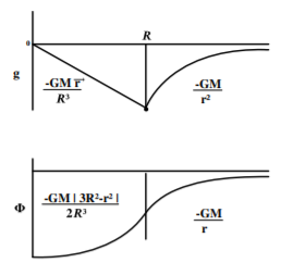
The field inside the Earth is radial and is proportional to the distance from the center of the Earth. This is Hooke’s Law, and thus ignoring air drag, any body dropped down a hole through the center of the Earth will undergo harmonic oscillations with an angular frequency of $\omega_0 = \sqrt{\frac{GM}{R^3}} = \sqrt{\frac{g}{R}}$. This gives a period of oscillation of 1.4 hours, which is about the length of a $P235$ lecture in classical mechanics, which may seem like a long time.

Clearly method (c) is much simpler to solve for this case. In general, look for a symmetry that allows identification of a surface upon which the magnitude and direction of the field is constant. For such cases use Gauss’s law. Otherwise use methods (a) or (b) whichever one is easiest to apply. Further examples will not be given here since they are essentially identical to those discussed extensively in electrostatics.