5.2: Euler’s Differential Equation

The calculus of variations, presented here, underlies the powerful variational approaches that were developed for classical mechanics. Variational calculus, developed for classical mechanics, now has become an essential approach to many other disciplines in science, engineering, economics, and medicine.

For the special case of one dimension, the calculus of variations reduces to varying the function $y(x)$ such that the scalar functional $F$ is an extremum, that is, it is a maximum or minimum, where.

$$F=\int_{x_{1}}^{x_{2}}f\left[ y(x),y^{\prime }(x);x\right] dx$$

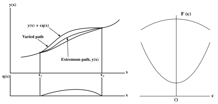
Here $x$ is the independent variable, $y(x)$ the dependent variable, plus its first derivative $y^{\prime }\equiv \frac{dy}{dx}$. The quantity $f\left[ y(x),y^{\prime }(x);x\right]$ has some given dependence on $y,y^{\prime }$ and $x.$ The calculus of variations involves varying the function $y(x)$ until a stationary value of $F$ is found, which is presumed to be an extremum. This means that if a function $y=y(x)$ gives a minimum value for the scalar functional $F$, then any neighboring function, no matter how close to $y(x),$ must increase $F$. For all paths, the integral $F$ is taken between two fixed points, $x_{1},y_{1}$ and $x_{2},y_{2}$. Possible paths between the initial and final points are illustrated in Figure $\PageIndex{1}$. Relative to any neighboring path, the functional $F$ must have a stationary value which is presumed to be the correct extremum path.

Define a neighboring function using a parametric representation $y(\epsilon ,x),$ such that for $\epsilon =0$, $y=y(0,x)=y(x)$ is the function that yields the extremum for $F$. Assume that an infinitesimally small fraction $\epsilon$ of the neighboring function $\eta (x)$ is added to the extremum path $y(x)$. That is, assume

$$\begin{align} y(\epsilon ,x) & = y(0,x)+\epsilon \eta (x) \label{5.4} \\[4pt] y^{\prime }(\epsilon ,x) & \equiv \frac{dy(\epsilon ,x)}{dx}=\frac{dy(0,x)}{ dx}+\epsilon \frac{d\eta }{dx} \notag\end{align}$$

where it is assumed that the extremum function $y(0,x)$ and the auxiliary function $\eta (x)$ are well behaved functions of $x$ with continuous first derivatives, and where $\eta (x)$ vanishes at $x_{1}$ and $x_{2},$ because, for all possible paths, the function $y(\epsilon ,x)$ must be identical with $y(x)$ at the end points of the path, i.e. $\eta (x_{1})=\eta (x_{2})=0$. The situation is depicted in Figure $\PageIndex{1}$. It is possible to express any such parametric family of curves $F$ as a function of $\epsilon$

$$F(\epsilon )=\int_{x_{1}}^{x_{2}}f\left[ y(\epsilon ,x),y^{\prime }(\epsilon ,x);x\right] dx \label{5.5}$$

The condition that the integral has a stationary (extremum) value is that $F$ be independent of $\epsilon$ to first order along the path. That is, the extremum value occurs for ($\epsilon =0$) where

$$\left( \frac{dF}{d\epsilon }\right) _{\epsilon =0}=0 \label{5.6}$$

for all functions $\eta (x).$ This is illustrated on the right side of Figure $\PageIndex{1}$.

Applying condition $\ref{5.6}$ to Equation $\ref{5.5}$, and since $x$ is independent of $\epsilon ,$ then

$$\frac{\partial F}{\partial \epsilon }=\int_{x_{1}}^{x_{2}}\left( \frac{ \partial f}{\partial y}\frac{\partial y}{\partial \epsilon }+\frac{\partial f }{\partial y^{\prime }}\frac{\partial y^{\prime }}{\partial \epsilon } \right) dx=0 \label{5.7}$$

Since the limits of integration are fixed, the differential operation affects only the integrand. From equations $\ref{5.4}$, $$\frac{\partial y}{\partial \epsilon }=\eta (x)$$

and $$\frac{\partial y^{\prime }}{\partial \epsilon }=\frac{d\eta }{dx}$$

Consider the second term in the integrand $$\int_{x_{1}}^{x_{2}}\frac{\partial f}{\partial y^{\prime }}\frac{\partial y^{\prime }}{\partial \epsilon }dx=\int_{x_{1}}^{x_{2}}\frac{\partial f}{ \partial y^{\prime }}\frac{d\eta }{dx}dx$$

Figure $\PageIndex{1}$: The left shows the extremum $y(x)$ and neighboring paths $y(\epsilon, x) = y(x) + \epsilon \eta (x)$ between $(x_1, y_1)$ and $(x_2, y_2)$ that minimizes the function $F = \int^{x_2}_{x_1} f[y(x), y^{\prime}(x); x] dx$. The right shows the dependence of $F$ as a function of the admixture coefficient $\epsilon$ for a maximum (upper) or a minimum (lower) at $\epsilon = 0$.

Integrate by parts

$$\int udv=uv-\int vdu$$ gives $$\int_{x_{1}}^{x_{2}}\frac{\partial f}{\partial y^{\prime }}\frac{d\eta }{dx} dx=\left[ \frac{\partial f}{\partial y^{\prime }}\eta (x)\right] _{x_{1}}^{x_{2}}-\int_{x_{1}}^{x_{2}}\eta (x)\frac{d}{dx}\left( \frac{ \partial f}{\partial y^{\prime }}\right) dx$$

Note that the first term on the right-hand side is zero since by definition $\frac{\partial y}{\partial \epsilon }=\eta (x)=0$ at $x_{1}$ and $x_{2}.$ Thus

$$\begin{align*} \frac{\partial F}{\partial \epsilon } &=\int_{x_{1}}^{x_{2}}\left( \frac{ \partial f}{\partial y}\frac{\partial y}{\partial \epsilon }+\frac{\partial f }{\partial y^{\prime }}\frac{\partial y^{\prime }}{\partial \epsilon } \right) dx \\[4pt] &=\int_{x_{1}}^{x_{2}}\left( \frac{\partial f}{\partial y}\eta (x)-\eta (x)\frac{d}{dx}\left( \frac{\partial f}{\partial y^{\prime }} \right) \right) dx \end{align*}$$

Thus Equation $\ref{5.7}$ reduces to

$$\frac{\partial F}{\partial \epsilon }=\int_{x_{1}}^{x_{2}}\left( \frac{ \partial f}{\partial y}-\frac{d}{dx}\frac{\partial f}{\partial y^{\prime }} \right) \eta (x)dx$$

The function $\frac{\partial F}{\partial \epsilon }$ will be an extremum if it is stationary at $\epsilon =0$. That is,

$$\frac{\partial F}{\partial \epsilon }=\int_{x_{1}}^{x_{2}}\left( \frac{ \partial f}{\partial y}-\frac{d}{dx}\frac{\partial f}{\partial y^{\prime }} \right) \eta (x)dx=0$$

This integral now appears to be independent of $\epsilon .$ However, the functions $y$ and $y^{\prime }$ occurring in the derivatives are functions of $\epsilon$. Since $\left( \frac{\partial F}{\partial \epsilon }\right) _{\epsilon =0}$ must vanish for a stationary value, and because $\eta (x)$ is an arbitrary function subject to the conditions stated , then the above integrand must be zero. This derivation that the integrand must be zero leads to Euler’s differential equation

$$\frac{\partial f}{\partial y}-\frac{d}{dx}\frac{\partial f}{\partial y^{\prime }}=0$$

where $y$ and $y^{\prime }$ are the original functions, independent of $\epsilon$. The basis of the calculus of variations is that the function $y(x)$ that satisfies Euler’s equation is an stationary function. Note that the stationary value could be either a maximum or a minimum value. When Euler’s equation is applied to mechanical systems using the Lagrangian as the functional, then Euler’s differential equation is called the Euler-Lagrange equation.