5.3: Applications of Euler’s Equation

Example \(\PageIndex{1}\): Shortest distance between two points

Consider the path lies in the \(\mathit{x-y}\) plane.

Figure \(\PageIndex{1}\): Shortest distance between two points in a plane.

The infinitessimal length of arc is

\[ds = \sqrt{dx^{2}+dy^{2}} = \left[ \sqrt{1+\left( \frac{dy}{dx}\right) ^{2}}\right] dx\nonumber\]

Then the length of the arc is \[J = \int_{1}^{2}ds = \int_{1}^{2}\left[ \sqrt{1+\left( \frac{dy}{dx}\right) ^{2}} \right] dx\nonumber\]

The function \(f\) is

\[f = \sqrt{1+\left( y^{\prime }\right) ^{2}}\nonumber\]

Therefore

\[\frac{\partial f}{\partial y} = 0\nonumber\]

and

\[\frac{\partial f}{\partial y^{\prime }} = \frac{y^{\prime }}{\sqrt{1+\left( y^{\prime }\right) ^{2}}}\nonumber\]

Inserting these into Euler’s equation \((5.2.13)\) gives

\[0+\frac{d}{dx}\left( \frac{y^{\prime }}{\sqrt{1+\left( y^{\prime }\right) ^{2}}}\right) = 0\nonumber\]

that is

\[\frac{y^{\prime }}{\sqrt{1+\left( y^{\prime }\right) ^{2}}} = \text{constant} = C\nonumber\]

This is valid if

\[y^{\prime } = \frac{C}{\sqrt{1-C^{2}}} = a\nonumber\]

Therefore

\[y = ax+b\nonumber\]

which is the equation of a straight line in the plane. Thus the shortest path between two points in a plane is a straight line between these points, as is intuitively obvious. This stationary value obviously is a minimum.

This trivial example of the use of Euler’s equation to determine an extremum value has given the obvious answer. It has been presented here because it provides a proof that a straight line is the shortest distance in a plane and illustrates the power of the calculus of variations to determine extremum paths.

Example \(\PageIndex{2}\): Brachistochrone problem

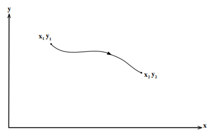
The Brachistochrone problem involves finding the path having the minimum transit time between two points. The Brachistochrone problem stimulated the development of the calculus of variations by John Bernoulli and Euler. For simplicity, take the case of frictionless motion in the \(x-y\) plane with a uniform gravitational field acting in the \( \widehat{\mathbf{y}}\) direction, as shown in the adjacent figure. The question is what constrained path will result in the minimum transit time between two points \((x_{1}y_{1})\) and \((x_{2}y_{2}).\)

Figure \(\PageIndex{2}\): The Bachistochrone problem involves finding the path for the minimum transit time for constrained frictionless motion in a uniform gravitational field.

Consider that the particle of mass \(m\) starts at the origin \(x_{1} = 0,y_{1} = 0\) with zero velocity. Since the problem conserves energy and assuming that initially \(E = KE+PE = 0\) then

\[\frac{1}{2}mv^{2}-mgy = 0\nonumber\]

That is \[v = \sqrt{2gy}\nonumber\]

The transit time is given by

\[t = \int_{x_{1}}^{x_{2}}\frac{ds}{v} = \int_{x_{1}}^{x_{2}}\frac{\sqrt{ dx^{2}+dy^{2}}}{\sqrt{2gy}} = \int_{x_{1}}^{x_{2}}\sqrt{\frac{\left( 1+x^{\prime 2}\right) }{2gy}}dy\nonumber\]

where \(x^{\prime }\equiv \frac{dx}{dy}\). Note that, in this example, the independent variable has been chosen to be \(y\) and the dependent variable is \(x(y)\).

The function \(f\) of the integral is

\[f = \frac{1}{\sqrt{2g}}\sqrt{\frac{\left( 1+x^{\prime 2}\right) }{y}}\nonumber\]

Factor out the constant \(\sqrt{2g}\) term, which does not affect the final equation, and note that

\[\begin{aligned} \frac{\partial f}{\partial x} & = &0 \\ \frac{\partial f}{\partial x^{\prime }} & = &\frac{x^{\prime }}{\sqrt{y\left( 1+\left( x^{\prime }\right) ^{2}\right) }}\end{aligned}\nonumber\]

Therefore Euler’s equation gives

\[0+\frac{d}{dy}\left( \frac{x^{\prime }}{\sqrt{y\left( 1+\left( x^{\prime }\right) ^{2}\right) }}\right) = 0\nonumber\]

or

\[\frac{x^{\prime }}{\sqrt{y\left( 1+\left( x^{\prime }\right) ^{2}\right) }} = \text{constant} = \frac{1}{\sqrt{2a}}\nonumber\]

That is

\[\frac{x^{\prime 2}}{y\left( 1+\left( x^{\prime }\right) ^{2}\right) } = \frac{1 }{2a}\nonumber\]

This may be rewritten as

\[x = \int_{y_{1}}^{y_{2}}\frac{ydy}{\sqrt{2ay-y^{2}}}\nonumber\]

Change the variable to \(y = a(1-\cos \theta )\) gives that \( dy = a\sin \theta d\theta ,\) leading to the integral

\[x = \int a\left( 1-\cos \theta \right) d\theta\nonumber\]

or

\[x = a(\theta -\sin \theta )+\text{constant}\nonumber\]

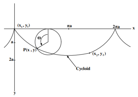
The parametric equations for a cycloid passing through the origin are

\[\begin{aligned} x & = &a(\theta -\sin \theta ) \\ y & = &a(1-\cos \theta )\end{aligned}\nonumber\]

which is the form of the solution found. That is, the shortest time between two points is obtained by constraining the motion of the mass to follow a cycloid shape. Thus the mass first accelerates rapidly by falling down steeply and then follows the curve and coasts upward at the end. The elapsed time is obtained by inserting the above parametric relations for \(x\) and \(y,\) in terms of \(\theta ,\) into the transit time integral giving \(t = \sqrt{\frac{a}{g}}\theta\) where\( \ a\) and \(\theta\) are fixed by the end point coordinates. Thus the time to fall from starting with zero velocity at the cusp to the minimum of the cycloid is \(\pi \sqrt{\frac{a}{g}}.\) If \(y_{2} = y_{1} = 0\) then \(x_{2} = 2\pi a\) which defines the shape of the cycloid and the minimum time is \(2\pi \sqrt{\frac{a}{g}} = \sqrt{ \frac{2\pi x_{2}}{g}}.\) If the mass starts with a non-zero initial velocity, then the starting point is not at the cusp of the cycloid, but down a distance \(d\) such that the kinetic energy equals the potential energy difference from the cusp.

A modern application of the Brachistochrone problem is determination of the optimum shape of the low-friction emergency chute that passengers slide down to evacuate a burning aircraft. Bernoulli solved the problem of rapid evacuation of an aircraft two centuries before the first flight of a powered aircraft.

Example \(\PageIndex{3}\): Minimal travel cost

Assume that the cost of flying an aircraft at height \(z\) is \(e^{-\kappa z}\) per unit distance of flight-path, where \( \kappa\) is a positive constant. Consider that the aircraft flies in the \((x,z)\)-plane from the point \((-a,0)\) to the point \((a,0)\) where \(z = 0\) corresponds to ground level, and where the \(z\)-axis points vertically upwards. Find the extremal for the problem of minimizing the total cost of the journey.

The differential arc-length element of the flight path \(ds\) can be written as

\[ds = \sqrt{dx^{2}+dz^{2}} = \sqrt{1+z^{\prime 2}}dx\nonumber\]

where \(z^{\prime }\equiv \frac{dz}{dx}\). Thus the cost integral to be minimized is

\[C = \int_{-a}^{+a}e^{-\kappa z}ds = \int_{-a}^{+a}e^{-\kappa z}\sqrt{1+z^{\prime 2}}dx\nonumber\]

The function of this integral is

\[f = e^{-\kappa z}\sqrt{1+z^{\prime 2}}\nonumber\]

The partial differentials required for the Euler equations are

\[\begin{aligned} \frac{d}{dx}\frac{\partial f}{\partial z^{\prime }} & = &\frac{z^{\prime \prime }e^{-\kappa z}}{\sqrt{1+z^{\prime 2}}}-\frac{\kappa z^{\prime 2}e^{-\kappa z}}{\sqrt{1+z^{\prime 2}}}-\frac{z^{\prime \prime }z^{\prime 2}e^{-\kappa z}}{\left( 1+z^{\prime 2}\right) ^{3/2}} \\ \frac{\partial f}{\partial z} & = &-\kappa e^{-\kappa z}\sqrt{1+z^{\prime 2}}\end{aligned}\nonumber\]

Therefore Euler’s equation equals

\[\frac{\partial f}{\partial z}-\frac{d}{dx}\frac{\partial f}{\partial z^{\prime }} = -\kappa e^{-\kappa z}\sqrt{1+z^{\prime 2}}-\frac{z^{\prime \prime }e^{-\kappa z}}{\sqrt{1+z^{\prime 2}}}+\frac{\kappa z^{\prime 2}e^{-\kappa z}}{\sqrt{1+z^{\prime 2}}}+\frac{z^{\prime \prime }z^{\prime 2}e^{-\kappa z}}{\left( 1+z^{\prime 2}\right) ^{3/2}} = 0\nonumber\]

This can be simplified by multiplying the radical to give

\[-\kappa -2\kappa z^{\prime 2}-\kappa z^{\prime 4}-z^{\prime \prime }-z^{\prime \prime }z^{\prime 2}+\kappa z^{\prime 2}+\kappa z^{\prime 4}+z^{\prime \prime }z^{\prime 2} = 0\nonumber\]

Cancelling terms gives

\[z^{\prime \prime }+\kappa \left( 1+z^{\prime 2}\right) = 0\nonumber\]

Separating the variables leads to

\[\arctan z^{\prime } = \int \frac{dz^{\prime }}{z^{\prime 2}+1} = -\int \kappa dx = -\kappa z+c_{1}\nonumber\]

Integration gives

\[z(x) = \int_{-a}^{x}dz = \int_{-a}^{x}\tan (c_{1}-\kappa x)dx = \frac{\ln (\cos (c_{1}-\kappa x))-\ln (\cos (c_{1}+\kappa a))}{\kappa }+c_{2} = \frac{\ln \left( \frac{\cos (c_{1}-\kappa x)}{\cos (c_{1}+\kappa a)}\right) }{\kappa } +c_{2}\nonumber\]

Using the initial condition that \(z(-a) = 0\) gives \(c_{2} = 0\). Similarly the final condition \(z(a) = 0\) implies that \( c_{1} = 0\). Thus Euler’s equation has determined that the optimal trajectory that minimizes the cost integral \(C\) is

\[z(x) = \frac{1}{\kappa }\ln \left( \frac{\cos (\kappa x)}{\cos (\kappa a)} \right)\nonumber\]

This example is typical of problems encountered in economics.