
7.10: Hamiltonian Invariance
- Page ID
- 14078

\( \newcommand{\vecs}[1]{\overset { \scriptstyle \rightharpoonup} {\mathbf{#1}} } \)
\( \newcommand{\vecd}[1]{\overset{-\!-\!\rightharpoonup}{\vphantom{a}\smash {#1}}} \)
\( \newcommand{\dsum}{\displaystyle\sum\limits} \)
\( \newcommand{\dint}{\displaystyle\int\limits} \)
\( \newcommand{\dlim}{\displaystyle\lim\limits} \)
\( \newcommand{\id}{\mathrm{id}}\) \( \newcommand{\Span}{\mathrm{span}}\)
( \newcommand{\kernel}{\mathrm{null}\,}\) \( \newcommand{\range}{\mathrm{range}\,}\)
\( \newcommand{\RealPart}{\mathrm{Re}}\) \( \newcommand{\ImaginaryPart}{\mathrm{Im}}\)
\( \newcommand{\Argument}{\mathrm{Arg}}\) \( \newcommand{\norm}[1]{\| #1 \|}\)
\( \newcommand{\inner}[2]{\langle #1, #2 \rangle}\)
\( \newcommand{\Span}{\mathrm{span}}\)
\( \newcommand{\id}{\mathrm{id}}\)
\( \newcommand{\Span}{\mathrm{span}}\)
\( \newcommand{\kernel}{\mathrm{null}\,}\)
\( \newcommand{\range}{\mathrm{range}\,}\)
\( \newcommand{\RealPart}{\mathrm{Re}}\)
\( \newcommand{\ImaginaryPart}{\mathrm{Im}}\)
\( \newcommand{\Argument}{\mathrm{Arg}}\)
\( \newcommand{\norm}[1]{\| #1 \|}\)
\( \newcommand{\inner}[2]{\langle #1, #2 \rangle}\)
\( \newcommand{\Span}{\mathrm{span}}\) \( \newcommand{\AA}{\unicode[.8,0]{x212B}}\)
\( \newcommand{\vectorA}[1]{\vec{#1}} % arrow\)
\( \newcommand{\vectorAt}[1]{\vec{\text{#1}}} % arrow\)
\( \newcommand{\vectorB}[1]{\overset { \scriptstyle \rightharpoonup} {\mathbf{#1}} } \)
\( \newcommand{\vectorC}[1]{\textbf{#1}} \)
\( \newcommand{\vectorD}[1]{\overrightarrow{#1}} \)
\( \newcommand{\vectorDt}[1]{\overrightarrow{\text{#1}}} \)
\( \newcommand{\vectE}[1]{\overset{-\!-\!\rightharpoonup}{\vphantom{a}\smash{\mathbf {#1}}}} \)
\( \newcommand{\vecs}[1]{\overset { \scriptstyle \rightharpoonup} {\mathbf{#1}} } \)
\(\newcommand{\longvect}{\overrightarrow}\)
\( \newcommand{\vecd}[1]{\overset{-\!-\!\rightharpoonup}{\vphantom{a}\smash {#1}}} \)
\(\newcommand{\avec}{\mathbf a}\) \(\newcommand{\bvec}{\mathbf b}\) \(\newcommand{\cvec}{\mathbf c}\) \(\newcommand{\dvec}{\mathbf d}\) \(\newcommand{\dtil}{\widetilde{\mathbf d}}\) \(\newcommand{\evec}{\mathbf e}\) \(\newcommand{\fvec}{\mathbf f}\) \(\newcommand{\nvec}{\mathbf n}\) \(\newcommand{\pvec}{\mathbf p}\) \(\newcommand{\qvec}{\mathbf q}\) \(\newcommand{\svec}{\mathbf s}\) \(\newcommand{\tvec}{\mathbf t}\) \(\newcommand{\uvec}{\mathbf u}\) \(\newcommand{\vvec}{\mathbf v}\) \(\newcommand{\wvec}{\mathbf w}\) \(\newcommand{\xvec}{\mathbf x}\) \(\newcommand{\yvec}{\mathbf y}\) \(\newcommand{\zvec}{\mathbf z}\) \(\newcommand{\rvec}{\mathbf r}\) \(\newcommand{\mvec}{\mathbf m}\) \(\newcommand{\zerovec}{\mathbf 0}\) \(\newcommand{\onevec}{\mathbf 1}\) \(\newcommand{\real}{\mathbb R}\) \(\newcommand{\twovec}[2]{\left[\begin{array}{r}#1 \\ #2 \end{array}\right]}\) \(\newcommand{\ctwovec}[2]{\left[\begin{array}{c}#1 \\ #2 \end{array}\right]}\) \(\newcommand{\threevec}[3]{\left[\begin{array}{r}#1 \\ #2 \\ #3 \end{array}\right]}\) \(\newcommand{\cthreevec}[3]{\left[\begin{array}{c}#1 \\ #2 \\ #3 \end{array}\right]}\) \(\newcommand{\fourvec}[4]{\left[\begin{array}{r}#1 \\ #2 \\ #3 \\ #4 \end{array}\right]}\) \(\newcommand{\cfourvec}[4]{\left[\begin{array}{c}#1 \\ #2 \\ #3 \\ #4 \end{array}\right]}\) \(\newcommand{\fivevec}[5]{\left[\begin{array}{r}#1 \\ #2 \\ #3 \\ #4 \\ #5 \\ \end{array}\right]}\) \(\newcommand{\cfivevec}[5]{\left[\begin{array}{c}#1 \\ #2 \\ #3 \\ #4 \\ #5 \\ \end{array}\right]}\) \(\newcommand{\mattwo}[4]{\left[\begin{array}{rr}#1 \amp #2 \\ #3 \amp #4 \\ \end{array}\right]}\) \(\newcommand{\laspan}[1]{\text{Span}\{#1\}}\) \(\newcommand{\bcal}{\cal B}\) \(\newcommand{\ccal}{\cal C}\) \(\newcommand{\scal}{\cal S}\) \(\newcommand{\wcal}{\cal W}\) \(\newcommand{\ecal}{\cal E}\) \(\newcommand{\coords}[2]{\left\{#1\right\}_{#2}}\) \(\newcommand{\gray}[1]{\color{gray}{#1}}\) \(\newcommand{\lgray}[1]{\color{lightgray}{#1}}\) \(\newcommand{\rank}{\operatorname{rank}}\) \(\newcommand{\row}{\text{Row}}\) \(\newcommand{\col}{\text{Col}}\) \(\renewcommand{\row}{\text{Row}}\) \(\newcommand{\nul}{\text{Nul}}\) \(\newcommand{\var}{\text{Var}}\) \(\newcommand{\corr}{\text{corr}}\) \(\newcommand{\len}[1]{\left|#1\right|}\) \(\newcommand{\bbar}{\overline{\bvec}}\) \(\newcommand{\bhat}{\widehat{\bvec}}\) \(\newcommand{\bperp}{\bvec^\perp}\) \(\newcommand{\xhat}{\widehat{\xvec}}\) \(\newcommand{\vhat}{\widehat{\vvec}}\) \(\newcommand{\uhat}{\widehat{\uvec}}\) \(\newcommand{\what}{\widehat{\wvec}}\) \(\newcommand{\Sighat}{\widehat{\Sigma}}\) \(\newcommand{\lt}{<}\) \(\newcommand{\gt}{>}\) \(\newcommand{\amp}{&}\) \(\definecolor{fillinmathshade}{gray}{0.9}\)Chapters \(7.8,7.9\) addressed two important and independent features of the Hamiltonian regarding: \(a)\) when \(H\) is conserved, and \(b\)) when \(H\) equals the total mechanical energy. These important results are summarized below with a discussion of the assumptions made in deriving the Hamiltonian, as well as the implications.
a) Conservation of generalized energy
The generalized energy theorem \((7.8.1)\) was given as
\[\dfrac{dH\left( \mathbf{q,p,}t\right) }{dt}=\dfrac{dh(\mathbf{q},\mathbf{\dot{q }},t)}{dt}=\sum_{j}\dot{q}_{j}\left[ Q_{j}^{EXC}+\sum_{k=1}^{m}\lambda _{k} \dfrac{\partial g_{k}}{\partial q_{j}}(\mathbf{q},t)\right] -\dfrac{\partial L( \mathbf{q},\mathbf{\dot{q}},t)}{\partial t} \label{7.46}\]
Note that when
\[\sum_{j}\dot{q}_{j}\left[ Q_{j}^{EXC}+\sum_{k=1}^{m}\lambda _{k}\dfrac{\partial g_{k}}{\partial q_{j}}(\mathbf{q},t)\right] =0, \nonumber\]
then Equation \ref{7.46} reduces to
\[\dfrac{dH}{dt}=-\dfrac{\partial L}{\partial t}\label{7.47}\]
Also, when
\[\sum_{j}\dot{q}_{j}\left[ Q_{j}^{EXC}+\sum_{k=1}^{m}\lambda _{k} \dfrac{\partial g_{k}}{\partial q_{j}}(\mathbf{q},t)\right] =0, \nonumber\]
and if the Lagrangian is not an explicit function of time, then the Hamiltonian is a constant of motion. That is, \(H\) is conserved if, and only if, the Lagrangian, and consequently the Hamiltonian, are not explicit functions of time, and if the external forces are zero.
b) The generalized energy and total energy
If the following two requirements are satisfied
- The kinetic energy has a homogeneous quadratic dependence on the generalized velocities, that is, the transformation to generalized coordinates is independent of time, \( \dfrac{\partial x_{\alpha ,i}}{\partial t}=0.\)
- The potential energy is not velocity dependent, thus the terms \(\dfrac{\partial U}{\partial \dot{q}_{i}}=0.\)
Then equation \((7.9.5)\) implies that the Hamiltonian equals the total mechanical energy, that is, \[H=T+U=E\label{7.48}\]
Expressed in words, the generalized energy (Hamiltonian) equals the total energy if the constraints are time independent and the potential energy is velocity independent. This is equivalent to stating that, if the constraints, or generalized coordinates, for the system are time independent, then \(H=E\).
The four combinations of the above two independent conditions, assuming that the external forces term in Equation \ref{7.46} is zero, are summarized in table \(\PageIndex{1}\).
| Hamiltonian | Constraints and coordinate transformation | Constraints and coordinate transformation |
|---|---|---|
| Time behavior | Time independent | Time dependent |
| \(\dfrac{dH}{dt}=-\dfrac{\partial L}{\partial t}=0\) | \(H\) conserved, \(H=E\) | \( H\) conserved, \(H\neq E\) |
| \(\dfrac{dH}{dt}=-\dfrac{\partial L}{\partial t}\neq 0\) | \(H\) not conserved, \( H=E\) | \(H\) not conserved, \(H\neq E\) |
Note the following general facts regarding the Lagrangian and the Hamiltonian.
- the Lagrangian is indefinite with respect to addition of a constant to the scalar potential,
- the Lagrangian is indefinite with respect to addition of a constant velocity,
- there is no unique choice of generalized coordinates.
- the Hamiltonian is a scalar function that is derived from the Lagrangian scalar function.
- the generalized momentum is derived from the Lagrangian.
These facts, plus the ability to recognize the conditions under which \(H\) is conserved, and when \(H=E,\) can greatly facilitate solving problems as shown by the following two examples.
Example \(\PageIndex{1}\): Linear harmonix oscillator on a cart moving at constant velocity
Consider a linear harmonic oscillator located on a cart that is moving with constant velocity \(v_{0}\) in the \(x\) direction (Figure \(\PageIndex{1}\)). Let the laboratory frame be the unprimed frame, and the cart frame be designated the primed frame. Assume that \(x=x^{\prime }\) at \(t=0.\) Then
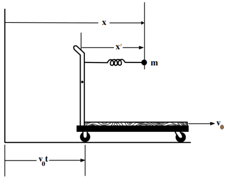
\[x^{\prime }=x-v_{0}t \hspace{0.85in}\dot{x}^{\prime }=\dot{x}-v_{0}\hspace{0.85in}\ddot{x} ^{\prime }=\ddot{x}\nonumber\]
The harmonic oscillator will have a potential energy of \[U=\dfrac{1}{2}kx^{\prime 2}=\dfrac{1}{2}k\left( x-v_{0}t\right) ^{2}\nonumber\]
Laboratory frame:
The Lagrangian is
\[L(x,\dot{x},t)=\dfrac{m\dot{x}^{2}}{2}-\dfrac{1}{2}k\left( x-v_{0}t\right) ^{2}\nonumber\]
Lagrange equation \(\Lambda _{x}L=0\) gives the equation of motion to be
\[m\ddot{x}=-k(x-v_{0}t) \nonumber\]
The definition of generalized momentum gives
\[p=\dfrac{\partial L}{\partial \dot{x}}=m\dot{x}\nonumber\]
The Hamiltonian is
\[\begin{align*} H(x,p,t) &=\sum_{i}\dot{q}_{i}\dfrac{\partial L}{\partial \dot{q}_{i}}-L \\[4pt] &=\dfrac{ p^{2}}{2m}+\dfrac{1}{2}k\left( x-v_{0}t\right) ^{2}\end{align*}\]
The Hamiltonian is the sum of the kinetic and potential energies and equals the total energy of the system, but it is not conserved since \(L\) and \(H\) are both explicit functions of time, that is \(\dfrac{dH}{dt}=\dfrac{\partial H}{\partial t}=-\dfrac{\partial L}{ \partial t}\neq 0\). Physically this is understood in that energy must flow into and out of the external constraint keeping the cart moving uniformly at a constant velocity \(v_{0}\) against the reaction to the oscillating mass. That is, assuming a uniform velocity for the moving cart constitutes a time-dependent constraint on the mass, and the force of constraint does work in actual displacement of the complete system. If the constraint did not exist, then the cart momentum would oscillate such that the total momentum of cart plus spring system is conserved.
Cart frame:
Transform the Lagrangian to the primed coordinates in the moving frame of reference, which also is an inertial frame. Then the Lagrangian \(L,\) in terms of the moving cart frame coordinates, is
\[L(x^{\prime },\dot{x}^{\prime },t)=\dfrac{m}{2}\left( \dot{x}^{\prime 2}+2 \dot{x}^{\prime }v_{0}+v_{0}^{2}\right) -\dfrac{1}{2}kx^{\prime 2}\nonumber\]
The Lagrange equation of motion \(\Lambda _{x^{\prime }}L=0\) gives the equation of motion to be
\[m\ddot{x}^{\prime }=-kx^{\prime }\nonumber\]
where \(x^{\prime }\) is the displacement of the mass with respect to the cart. This implies that an observer on the cart will observe simple harmonic motion as is to be expected from the principle of equivalence in Galilean relativity.
The definition of the generalized momentum gives the linear momentum in the primed frame coordinates to be
\[p^{\prime }=\dfrac{\partial L}{\partial \dot{x}^{\prime }}=m\dot{x}^{\prime }+mv_{0}\nonumber\]
The cart-frame Hamiltonian also can be expressed in terms of the coordinates in the moving frame to be
\[H(x^{\prime },p^{\prime },t)=\dot{x}^{\prime }\dfrac{\partial L}{\partial \dot{x}^{\prime }}-L=\dfrac{\left( p^{\prime }-mv_{0}\right) ^{2}}{2m}+\dfrac{1 }{2}kx^{\prime 2}-\dfrac{m}{2}v_{0}^{2}\nonumber\]
Note that the Lagrangian and Hamiltonian expressed in terms of the coordinates in the cart frame of reference are not explicitly time dependent, therefore \(H\) is conserved. However, the cart-frame Hamiltonian does not equal the total energy since the coordinate transformation is time dependent. Actually the first two terms in the above Hamiltonian are the energy of the harmonic oscillator in the cart frame. This example shows that the Hamiltonians differ when expressed in terms of either the laboratory or cart frames of reference
Example \(\PageIndex{2}\): Isotropic central force in a rotating frame
Consider a mass subject to a central isotropic radial force \(U(r)\) as shown in Figure \(\PageIndex{2}\). Compare the Hamiltonian \(H\) in the fixed frame of reference \(S\), with the Hamiltonian \(H^{\prime }\) in a frame of reference \(S^{\prime }\) that is rotating about the center of the force with constant angular velocity \( \omega\).
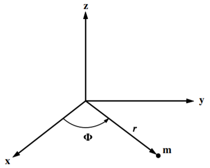
Restrict this case to rotation about one axis so that only two polar coordinates \(r\) and \(\phi\) need to be considered. The transformations are
\[\begin{aligned} r^{\prime } &=&r \\ \phi ^{\prime } &=&\phi -\omega t\end{aligned}\]
Also
\[U(r)=U(r^{\prime })\nonumber\]
Fixed frame of reference \(S\):
\[L=T-U= \dfrac{m}{2}\left( \dot{r}^{2}+r^{2}\dot{\phi}^{2}\right) -U(r)\nonumber\] Since the Lagrangian is not explicitly time dependent, then the Hamiltonian is conserved. For this fixed-frame Hamiltonian the generalized momenta are
\[\begin{aligned} p_{\phi } &=&\dfrac{\partial L}{\partial \dot{\phi}}=m\dot{r}^{2}\dot{\phi} \\ p_{r} &=&\dfrac{\partial L}{\partial \dot{r}}=m\dot{r}\end{aligned}\]
The Hamiltonian equals
\[H(p_{r},p_{\phi },r,\phi )=\sum_{i}\dot{q}_{i}\dfrac{\partial L}{\partial \dot{q}_{i}}-L=\dfrac{1}{2m}\left( p_{r}^{2}+\dfrac{p_{\phi }}{r^{2}} ^{2}\right) +U(r)=E \nonumber\]
The Hamiltonian in the fixed frame is conserved and equals the total energy, that is \(H=T+U\).
Rotating frame of reference \(S^{\prime }\)
The above inertial fixed-frame Lagrangian can be written in terms of the primed (non-inertial rotating frame) coordinates as
\[L=T-U=\dfrac{m}{2}\left( \dot{r}^{2}+r^{2}\dot{\phi}^{2}\right) -U(r)=\dfrac{m }{2}\left( \dot{r}^{\prime 2}+r^{\prime 2}\left( \dot{\phi}^{\prime }+\omega \right) ^{2}\right) -U(r^{\prime })\nonumber\]
The generalized momenta derived from this Lagrangian are
\[\begin{aligned} p_{\phi }^{\prime } &=&\dfrac{\partial L}{\partial \dot{\phi}^{\prime }}=m \dot{r}^{\prime 2}\left( \dot{\phi}^{\prime }+\omega \right) =p_{\phi ^{\prime }}^{\prime }+mr^{\prime 2}\omega \\ p_{r}^{\prime } &=&\dfrac{\partial L}{\partial \dot{r}^{\prime }}=m\dot{r} ^{\prime 2}=p_{r}\end{aligned}\]
The Hamiltonian expressed in terms of the non-inertial rotating frame coordinates is
\[H^{\prime }(p_{r}^{\prime },p_{\phi }^{\prime },r^{\prime },\phi ^{\prime })= \dfrac{\partial L}{\partial \dot{r}^{\prime }}\dot{r}^{\prime }+\dfrac{ \partial L}{\partial \dot{\phi}^{\prime }}\dot{\phi}^{\prime }-L=\dfrac{1}{2m} \left( p_{r}^{\prime 2}+\dfrac{\left( p_{\phi ^{\prime }}^{\prime }+mr^{2}\omega \right) }{r^{2}}\right) +U(r^{\prime })\nonumber\]
Note that \(H^{\prime }(p_{r}^{\prime },p_{\phi }^{\prime },r^{\prime },\phi ^{\prime })\) is time independent and therefore is conserved, but \(H(p_{r}^{\prime },p_{\phi }^{\prime },r^{\prime },\phi ^{\prime })\neq E\) because the generalized coordinates are time dependent. In addition, \(p_{\phi ^{\prime }}^{\prime }\) is conserved since \[\dot{p}_{\phi }^{\prime }=\dfrac{\partial H}{\partial \phi ^{\prime }}=-\dfrac{ \partial L}{\partial \phi ^{\prime }}=0\nonumber\]
Example \(\PageIndex{3}\): The plane pendulum
The simple plane pendulum in a uniform gravitational field \(g\) is an example that illustrates Hamiltonian invariance.
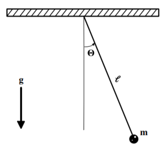
There is only one generalized coordinate, \(\theta\) and the Lagrangian for this system is
\[L= \dfrac{1}{2}ml^{2}\dot{\theta}^{2}+mgl\cos \theta \nonumber\]
The momentum conjugate to \(\theta\) is
\[p_{\theta }=\dfrac{\partial L}{\partial \dot{\theta}}=ml^{2}\dot{\theta} \nonumber\] which is the angular momentum about the pivot point.
Using the Lagrange-Euler equation this gives that
\[\dfrac{d}{dt}p_{\theta }=\dot{p}_{\theta }=\dfrac{\partial L}{\partial \theta } =-mgl\sin \theta \nonumber\] Note that the angular momentum \(p_{\theta }\) is not a constant of motion since it explicitly depends on \(\theta\).
The Hamiltonian is \[H=\sum_{i}p_{i}\dot{q}_{i}-L=p_{\theta }\dot{\theta}-L=\dfrac{1}{2}ml^{2}\dot{ \theta}^{2}-mgl\cos \theta =\dfrac{p_{\theta }^{2}}{2ml^{2}}-mgl\cos \theta \nonumber\]
Note that the Lagrangian and Hamiltonian are not explicit functions of time, therefore they are conserved. Also the potential is velocity independent and there is no coordinate transformation, thus the Hamiltonian equals the total energy \(E,\) which is a constant of motion. \[H=\dfrac{p_{\theta }^{2}}{2ml^{2}}-mgl\cos \theta =E \nonumber\]
Example \(\PageIndex{4}\): Oscillating cylinder in a cylindrical bowl
It is important to correctly account for constraint forces when using Noether’s theorem for constrained systems. Noether’s theorem assumes the variables are independent. This is illustrated by considering the example of a solid cylinder rolling in a fixed cylindrical bowl. Assume that a uniform cylinder of radius \(\rho\) and mass \(m\) is constrained to roll without slipping on the inner surface of the lower half of a hollow cylinder of radius \(R\). The motion is constrained to ensure that the axes of both cylinders remain parallel and \( \rho <R\).
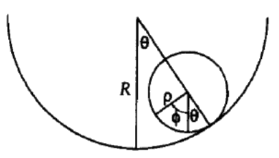
The generalized coordinates are taken to be the angles \(\theta\) and \(\phi\) which are measured with respect to a fixed vertical axis. Then the kinetic energy and potential energy are
\[T=\dfrac{1}{2}m\left[ \left( R-\rho \right) \dot{\theta}\right] ^{2}+\dfrac{1}{ 2}I\dot{\phi}^{2}\hspace{1in}U=\left[ R-\left( R-\rho \right) \cos \theta \right] mg \nonumber\]
where \(m\) is the mass of the small cylinder and where \( U=0\) at the lowest position of the sphere. The moment of inertia of a uniform cylinder is \(I=\dfrac{1}{2}m\rho ^{2}\).
The Lagrangian is
\[L-T-U=\dfrac{1}{2}m\left[ \left( R-\rho \right) \dot{\theta}\right] ^{2}+ \dfrac{1}{4}m\rho ^{2}\dot{\phi}^{2}-\left[ R-\left( R-\rho \right) \cos \theta \right] mg \nonumber\]
Since the solid cylinder rotates without slipping inside the cylindrical shell, then the equation of constraint is \[g(\theta \phi )=R\theta -\rho \left( \phi +\theta \right) =0 \nonumber\]
Using the Lagrangian, plus the one equation of constraint, requires one Lagrange multiplier. Then the Lagrange equations of motion for \(\theta\) and \(\phi\) are
\[\begin{aligned} \dfrac{\partial L}{\partial \theta }-\dfrac{d}{dt}\left[ \dfrac{\partial L}{ \partial \dot{\theta}}\right] +\lambda \dfrac{\partial g}{\partial \theta } &=&0 \\ \dfrac{\partial L}{\partial \phi }-\dfrac{d}{dt}\left[ \dfrac{\partial L}{ \partial \dot{\phi}}\right] +\lambda \dfrac{\partial g}{\partial \phi } &=&0\end{aligned}\]
Substitute the Lagrangian and the equation of constraint gives two equations of motion
\[\begin{aligned} -\left( R-\rho \right) mg\sin \theta -m\left( R-\rho \right) ^{2}\ddot{\theta }+\lambda \left( R-\rho \right) &=&0 \\ -\dfrac{1}{2}m\rho ^{2}\ddot{\phi}-\lambda \rho &=&0\end{aligned}\]
The lower equation of motion gives that
\[\lambda =-\dfrac{1}{2}m\rho \ddot{\phi} \nonumber\]
Substitute this into the equation of constraint gives
\[\lambda =-\dfrac{1}{2}m\left( R-\rho \right) \ddot{\theta} \nonumber\]
Substitute this into the first equation of motion gives the equation of motion for \(\theta\) to be
\[\ddot{\theta}=\dfrac{2g}{3\left( R-\rho \right) }\sin \theta\nonumber\]
that is
\[\lambda =-\dfrac{mg}{3}\sin \theta\nonumber\]
The torque acting on the small cylinder due to the frictional force is
\[F\rho =\dfrac{1}{2}m\rho ^{2}\ddot{\phi}=-\lambda \rho\nonumber\]
Thus the frictional force is \[F=-\lambda =\dfrac{mg}{3}\sin \theta\nonumber\]
Noether’s theorem can be used to ascertain if the angular momentum \( p_{\theta }\) is a constant of motion. The derivative of the Lagrangian
\[\dfrac{\partial L}{\partial \theta }=\left( R-\rho \right) mg\sin \theta\nonumber\]
and thus the Lagrange equations tells us that \(\dot{p}_{\theta }=\left( R-\rho \right) mg\sin \theta\). Therefore \(p_{\theta }\) is not a constant of motion.
The Lagrangian is not an explicit function of \(\phi ,\) which would suggest that \(p_{\phi }\) is a constant of motion. But this is incorrect because the constraint equation \(\phi =\dfrac{\left( R-\rho \right) }{\rho }\theta\) couples \(\theta\) and \( \phi\), that is, they are not independent variables, and thus \( p_{\theta }\) and \(p_{\phi }\) are coupled by the constraint equation. As a result \(p_{\phi }\) is not a constant of motion because it is directly coupled to \(p_{\theta }=\left( R-\rho \right) mg\sin \theta\) which is not a constant of motion. Thus neither \(p_{\theta }\) nor \(p_{\phi }\) are constants of motion. This illustrates that one must account carefully for equations of constraint, and the concomitant constraint forces, when applying Noether’s theorem which tacitly assumes independent variables.
The Hamiltonian can be derived using the generalized momenta
\[\begin{aligned} p_{\theta } &=&\dfrac{\partial L}{\partial \dot{\theta}}=m\left( R-\rho \right) ^{2}\dot{\theta} \\ p_{\phi } &=&\dfrac{\partial L}{\partial \dot{\phi}}=\dfrac{1}{2}m\rho ^{2} \dot{\phi}\end{aligned}\]
Then the Hamiltonian is given by
\[H=p_{\theta }\dot{\theta}+p_{\phi }\dot{\phi}-L=\dfrac{p_{\theta }^{2}}{ 2m\left( R-\rho \right) ^{2}}+\dfrac{p_{\phi }^{2}}{m\rho ^{2}}+\left[ R-\left( R-\rho \right) \cos \theta \right] mg\nonumber\]
Note that the transformation to generalized coordinates is time independent and the potential is not velocity dependent, thus the Hamiltonian also equals the total energy. Also the Hamiltonian is conserved since \(\dfrac{dH}{dt}=0\).