10.4: Rayleigh’s Dissipation Function

As mentioned above, nonconservative systems involving viscous or frictional dissipation, typically result from weak thermal interactions with many nearby atoms, making it impractical to include a complete set of active degrees of freedom. In addition, dissipative systems usually involve complicated dependences on the velocity and surface properties that are best handled by including the dissipative drag force explicitly as a generalized drag force in the Euler-Lagrange equations. The drag force can have any functional dependence on velocity, position, or time.

$$\mathbf{F}^{drag}=-f(\mathbf{\dot{q}},\mathbf{q},t)\mathbf{\hat{v}}$$

Note that since the drag force is dissipative the dominant component of the drag force must point in the opposite direction to the velocity vector.

In $1881$ Lord Rayleigh showed that if a dissipative force $\mathbf{F}$ depends linearly on velocity, it can be expressed in terms of a scalar potential functional of the generalized coordinates called the Rayleigh dissipation function $\mathcal{R(}\mathbf{\dot{q})}$. The Rayleigh dissipation function is an elegant way to include linear velocity-dependent dissipative forces in both Lagrangian and Hamiltonian mechanics, as is illustrated below for both Lagrangian and Hamiltonian mechanics.

Generalized dissipative forces for linear velocity dependence

Consider $n$ equations of motion for the $n$ degrees of freedom, and assume that the dissipation depends linearly on velocity. Then, allowing all possible cross coupling of the equations of motion for $q_{j},$ the equations of motion can be written in the form

$$\sum_{i=1}^{n}\left[ m_{ij} \ddot{q}_{j}+b_{ij}\dot{q}_{j}+c_{ij}q_{j}-Q_{i}(t)\right] =0 \label{10.5}$$

Multiplying Equation $\ref{10.5}$ by $\dot{q}_{i}$, take the time integral, and sum over $i,j$, gives the following energy equation

$$\sum_{i=1}^{n}\sum_{j=1}^{n}\int_{0}^{t}m_{ij}\ddot{q}_{j}\dot{q} _{i}dt+\sum_{i=1}^{n}\sum_{j=1}^{n}\int_{0}^{t}b_{ij}\dot{q}_{j}\dot{q} _{i}dt+\sum_{i=1}^{n}\sum_{j=1}^{n}\int_{0}^{t}c_{ij}q_{j}\dot{q} _{i}dt=\sum_{i}^{n}\int_{0}^{t}Q_{i}(t)\dot{q}_{i}dt$$

The right-hand term is the total energy supplied to the system by the external generalized forces $Q_{i}(t)$ at the time $t$. The first time-integral term on the left-hand side is the total kinetic energy, while the third time-integral term equals the potential energy. The second integral term on the left is defined to equal $2\mathcal{R}(\mathbf{\dot{q}} )$ where Rayeigh’s dissipation function $\mathcal{R}(\mathbf{\dot{q}})$ is defined as

$$\mathcal{R}(\mathbf{ \dot{q}})\mathcal{\equiv }\frac{1}{2}\sum_{i=1}^{n}\sum_{j=1}^{n}b_{ij}\dot{q }_{i}\dot{q}_{j}$$

and the summations are over all $n$ particles of the system. This definition allows for complicated cross-coupling effects between the $n$ particles.

The particle-particle coupling effects usually can be neglected allowing use of the simpler definition that includes only the diagonal terms. Then the diagonal form of the Rayleigh dissipation function simplifies to

$$\mathcal{R}(\mathbf{\dot{q}})\mathcal{\equiv }\frac{1}{2}\sum_{i=1}^{n}b_{i} \dot{q}_{i}^{2}$$

Therefore the frictional force in the $q_{i}$ direction depends linearly on velocity $\dot{q}_{i}$, that is

$$F_{q_{i}}^{f}=-\frac{\partial \mathcal{R}(\mathbf{\dot{q}})}{\partial \dot{q} _{i}}=-b_{i}\dot{q}_{i}$$

In general, the dissipative force is the velocity gradient of the Rayleigh dissipation function,

$$\mathbf{F}^{f}=-\nabla _{\mathbf{\dot{q}}}\mathcal{R}(\mathbf{\dot{q}})$$

The physical significance of the Rayleigh dissipation function is illustrated by calculating the work done by one particle $i$ against friction, which is

$$dW_{i}^{f}=-\mathbf{F}_{i}^{f}\cdot d\mathbf{r=-F}_{i}^{f}\cdot \mathbf{\dot{ q}}_{i}dt=b_{i}\dot{q}_{i}^{2}dt$$ Therefore

$$2\mathcal{R}(\mathbf{\dot{q}})\mathcal{=}\frac{dW^{f}}{dt}$$

which is the rate of energy (power) loss due to the dissipative forces involved. The same relation is obtained after summing over all the particles involved.

Transforming the frictional force into generalized coordinates requires equation $(6.3.10)$

$$\mathbf{\dot{r}}_{i}\mathbf{=}\sum_{k}\frac{\partial \mathbf{r}_{i}}{ \partial q_{k}}\dot{q}_{k}+\frac{\partial \mathbf{r}_{i}}{\partial t}$$

Note that the derivative with respect to $\dot{q}_{k}$ equals

$$\frac{\partial \mathbf{\dot{r}}_{i}}{\partial \dot{q}_{j}}=\frac{\partial \mathbf{r}_{i}}{\partial q_{j}}$$

Using equations $(6.3.11)$ and $7.3.12$, the $j$ component of the generalized frictional force $Q_{j}^{f}$ is given by

$$Q_{j}^{f}=\sum_{i=1}^{n}\mathbf{F}_{i}^{f}\cdot \frac{\partial \mathbf{r}_{i} }{\partial q_{j}}=\sum_{i=1}^{n}\mathbf{F}_{i}^{f}\cdot \frac{\partial \mathbf{\dot{r}}_{i}}{\partial \dot{q}_{j}}=-\sum_{i=1}^{n}\nabla _{v_{i}} \mathcal{R}(\mathbf{\dot{q}})\cdot \frac{\partial \mathbf{\dot{r}}_{i}}{ \partial \dot{q}_{j}}=-\frac{\partial \mathcal{R}(\mathbf{\dot{q}})}{ \partial \dot{q}_{j}}\label{10.15}$$

Equation $\ref{10.15}$ provides an elegant expression for the generalized dissipative force $Q_{j}^{f}$ in terms of the Rayleigh’s scalar dissipation potential $\mathcal{R}$.

Generalized dissipative forces for nonlinear velocity dependence

The above discussion of the Rayleigh dissipation function was restricted to the special case of linear velocity-dependent dissipation. Virga[Vir15] proposed that the scope of the classical Rayleigh-Lagrange formalism can be extended to include nonlinear velocity dependent dissipation by assuming that the nonconservative dissipative forces are defined by

$$\mathbf{F}_{i}^{f}=-\frac{\partial R(\mathbf{q},\mathbf{\dot{q}})}{\partial \mathbf{\dot{q}}}$$

where the generalized Rayleigh dissipation function $\mathcal{R(}\mathbf{q}, \mathbf{\dot{q}})$ satisfies the general Lagrange mechanics relation

$$\frac{\delta L}{\delta q}-\frac{\partial R}{\partial \dot{q}}=0$$

This generalized Rayleigh’s dissipation function eliminates the prior restriction to linear dissipation processes, which greatly expands the range of validity for using Rayleigh’s dissipation function.

Lagrange equations of motion

Linear dissipative forces can be directly, and elegantly, included in Lagrangian mechanics by using Rayleigh’s dissipation function as a generalized force $Q_{j}^{f}$. Inserting Rayleigh dissipation function $\ref{10.15}$ in the generalized Lagrange equations of motion $(6.5.12)$ gives

$$\left\{ \frac{d}{dt}\left( \frac{\partial L}{\partial \dot{q}_{j}}\right) - \frac{\partial L}{\partial q_{j}}\right\} =\left[ \sum_{k=1}^{m}\lambda _{k} \frac{\partial g_{k}}{\partial q_{j}}(\mathbf{q},t)+Q_{j}^{EXC}\right] - \frac{\partial \mathcal{R(}\mathbf{q},\mathbf{\dot{q}})}{\partial \dot{q}_{j} }\label{10.18}$$

where $Q_{j}^{EXC}$ corresponds to the generalized forces remaining after removal of the generalized linear, velocity-dependent, frictional force $Q_{j}^{f}$.

The holonomic forces of constraint are absorbed into the Lagrange multiplier term.

Hamiltonian mechanics

If the nonconservative forces depend linearly on velocity, and are derivable from Rayleigh’s dissipation function according to Equation $\ref{10.15}$, then using the definition of generalized momentum gives

$$\begin{align} \dot{p}_{i} &=&\frac{d}{dt}\frac{\partial L}{\partial \dot{q}_{j}}=\frac{ \partial L}{\partial q_{i}}+\left[ \sum_{k=1}^{m}\lambda _{k}\frac{\partial g_{k}}{\partial q_{j}}(\mathbf{q},t)+Q_{j}^{EXC}\right] -\frac{\partial \mathcal{R(}\mathbf{q},\mathbf{\dot{q}})}{\partial \dot{q}_{j}} \\ \dot{p}_{i} &=&-\frac{\partial H(\mathbf{p,q},t\mathbf{)}}{\partial q_{i}}+ \left[ \sum_{k=1}^{m}\lambda _{k}\frac{\partial g_{k}}{\partial q_{j}}( \mathbf{q},t)+Q_{j}^{EXC}\right] -\frac{\partial \mathcal{R(}\mathbf{q}, \mathbf{\dot{q}})}{\partial \dot{q}_{j}}\end{align}$$

Thus Hamilton’s equations become

$$\begin{align} \dot{q}_{i} &=&\frac{\partial H}{\partial p_{i}} \\ \dot{p}_{i} &=&-\frac{\partial H}{\partial q_{i}}+\left[ \sum_{k=1}^{m} \lambda _{k}\frac{\partial g_{k}}{\partial q_{j}}(\mathbf{q},t)+Q_{j}^{EXC} \right] -\frac{\partial \mathcal{R(}\mathbf{q},\mathbf{\dot{q}})}{\partial \dot{q}_{j}}\end{align}$$

The Rayleigh dissipation function $\mathcal{R(}\mathbf{q},\mathbf{\dot{q}})$ provides an elegant and convenient way to account for dissipative forces in both Lagrangian and Hamiltonian mechanics.

Example $\PageIndex{1}$: Driven, Linearly-Damped, Coupled Linear Oscillators

Consider the two identical, linearly damped, coupled oscillators (damping constant $\beta$) shown in the figure.

Figure $\PageIndex{1}$: Harmonically-driven, linearly-damped, coupled linear oscillators.

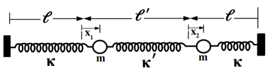
A periodic force $F=F_{0}\cos (\omega t)$ is applied to the left-hand mass $m$. The kinetic energy of the system is

$$T=\frac{1}{2}m(\dot{x}_{1}^{2}+\dot{x}_{2}^{2})\nonumber$$ The potential energy is

$$U=\frac{1}{2}\kappa x_{1}^{2}+\frac{1}{2}\kappa x_{2}^{2}+\frac{1}{2}\kappa ^{\prime }\left( x_{2}-x_{1}\right) ^{2}=\frac{1}{2}\left( \kappa +\kappa ^{\prime }\right) x_{1}^{2}+\frac{1}{2}\left( \kappa +\kappa ^{\prime }\right) x_{2}^{2}-\kappa ^{\prime }x_{1}x_{2} \notag$$

Thus the Lagrangian equals

$$L=\frac{1}{2}m(\dot{x}_{1}^{2}+\dot{x}_2^{2})-\left[ \frac{1}{2} ( \kappa +\kappa^{\prime } ) x_{1}^{2}+\frac{1}{2} ( \kappa +\kappa^{\prime } ) x_{2}^{2}-\kappa^{\prime }x_{1}x_{2}\right]\nonumber$$

Since the damping is linear, it is possible to use the Rayleigh dissipation function

$$\mathcal{R=}\frac{1}{2}\beta (\dot{x}_{1}^{2}+\dot{x}_{2}^{2})\nonumber$$

The applied generalized forces are

$$Q_{1}^{\prime }=F_{o}\cos \left( \omega t\right) \hspace{1in}Q_{2}^{\prime }=0\nonumber$$

Use the Euler-Lagrange equations $\ref{10.18}$ to derive the equations of motion

$$\left\{ \frac{d}{dt}\left( \frac{\partial L}{\partial \dot{q}_{j}}\right) - \frac{\partial L}{\partial q_{j}}\right\} +\frac{\partial \mathcal{F}}{ \partial \dot{q}_{j}}=Q_{j}^{\prime }+\sum_{k=1}^{m}\lambda _{k}\frac{ \partial g_{k}}{\partial q_{j}}(\mathbf{q},t)\nonumber$$ gives $$\begin{aligned} m\ddot{x}_{1}+\beta \dot{x}_{1}+(\kappa +\kappa ^{\prime })x_{1}-\kappa ^{\prime }x_{2} &=&F_{0}\cos \left( \omega t\right) \\ m\ddot{x}_{2}+\beta \dot{x}_{2}+(\kappa +\kappa ^{\prime })x_{2}-\kappa ^{\prime }x_{1} &=&0\end{aligned}$$

These two coupled equations can be decoupled and simplified by making a transformation to normal coordinates, $\eta _{1},\eta _{2}$ where

$$\eta _{1}=x_{1}-x_{2}\hspace{1in}\eta _{2}=x_{1}+x_{2}\nonumber$$

Thus

$$x_{1}=\frac{1}{2}(\eta _{1}+\eta _{2})\hspace{1in}x_{2}=\frac{1}{2}(\eta _{2}-\eta _{1})\nonumber$$

Insert these into the equations of motion gives

$$\begin{aligned} m(\ddot{\eta}_{1}+\ddot{\eta}_{2})+\beta (\dot{\eta}_{1}+\dot{\eta} _{2})+(\kappa +\kappa ^{\prime })(\eta _{1}+\eta _{2})-\kappa ^{\prime }(\eta _{2}-\eta _{1}) &=&2F_{0}\cos \left( \omega t\right) \\ m(\eta _{2}-\eta _{1})+\beta (\eta _{2}-\eta _{1})+(\kappa +\kappa ^{\prime })(\eta _{2}-\eta _{1})-\kappa ^{\prime }(\eta _{1}+\eta _{2}) &=&0\end{aligned}$$

Add and subtract these two equations gives the following two decoupled equations

$$\begin{aligned} \ddot{\eta}_{1}+\frac{\beta }{m}\dot{\eta}_{1}+\frac{\left( \kappa +2\kappa ^{\prime }\right) }{m}\eta _{1} &=&\frac{F_{0}}{m}\cos \left( \omega t\right) \\ \ddot{\eta}_{2}+\frac{\beta }{m}\dot{\eta}_{2}+\frac{\kappa }{m}\eta _{2} &=& \frac{F_{0}}{m}\cos \left( \omega t\right)\end{aligned}$$

Define $\Gamma =\frac{\beta }{m},\omega _{1}=\sqrt{\frac{\left( \kappa +2\kappa ^{\prime }\right) }{m}},\omega _{2}=\sqrt{\frac{\kappa }{m}} ,A=\frac{F_{0}}{m}$. Then the two independent equations of motion become

$$\ddot{\eta}_{1}+\Gamma \dot{\eta}_{1}+\omega _{1}^{2}\eta _{1}=A\cos \left( \omega t\right) \hspace{1in}\ddot{\eta}_{2}+\Gamma \dot{\eta}_{2}+\omega _{2}^{2}\eta _{2}=A\cos \left( \omega t\right)\nonumber$$

This solution is a superposition of two independent, linearly-damped, driven normal modes $\eta _{1}$ and $\eta _{2}$ that have different natural frequencies $\omega _{1}$ and $\omega _{2}$. For weak damping these two driven normal modes each undergo damped oscillatory motion with the $\eta _{1}$ and $\eta _{2}$ normal modes exhibiting resonances at $\omega _{1}^{\prime }=\sqrt{\omega _{1}^{2}-2\left( \frac{\Gamma }{2}\right) ^{2}}$ and $\omega _{2}^{\prime }=\sqrt{\omega _{2}^{2}-2\left( \frac{ \Gamma }{2}\right) ^{2}}$

Example $\PageIndex{2}$: Kirchhoff’s Rules for Electrical Circuits

The mathematical equations governing the behavior of mechanical systems and $LRC$ electrical circuits have a close similarity. Thus variational methods can be used to derive the analogous behavior for electrical circuits. For example, for a system of $n$ separate circuits, the magnetic flux $\Phi _{ik \text{ }}$through circuit $i,$ due to electrical current $I_{k}=\dot{q}_{k}$ flowing in circuit $k,$ is given by

$$\Phi _{ik}=M_{ik}\dot{q}_{k}\nonumber$$

where $M_{ik}$ is the mutual inductance. The diagonal term $M_{ii}=L_{i}$ corresponds to the self inductance of circuit $i$. The net magnetic flux $\Phi _{i}$ through circuit $i,$ due to all $n$ circuits, is the sum

$$\Phi _{i}=\sum_{k=1}^{n}M_{ik}\dot{q}_{k}\nonumber$$

Thus the total magnetic energy $W_{mag},$which is analogous to kinetic energy $T,$ is given by summing over all $n$ circuits to be

$$W_{mag}=T=\frac{1}{2}\sum_{i=1}^{n}\sum_{k=1}^{n}M_{ik}\dot{q}_{i}\dot{q}_{k}\nonumber$$

Similarly the electrical energy $W_{elect}$ stored in the mutual capacitance $C_{ik}$ between the $n$ circuits, which is analogous to potential energy, $U,$ is given by

$$W_{elect}=U=\frac{1}{2}\sum_{i=1}^{n}\sum_{k=1}^{n}\frac{q_{i}q_{k}}{C_{ik}}\nonumber$$

Thus the standard Lagrangian for this electric system is given by

$$L=T-U=\frac{1}{2}\sum_{i=1}^{n}\sum_{k=1}^{n}\left[ M_{ik}\dot{q}_{i}\dot{q} _{k}-\frac{q_{i}q_{k}}{C_{ik}}\right] \tag{$\alpha $} \label{alpha}$$

Assuming that Ohm’s Law is obeyed, that is, the dissipation force depends linearly on velocity, then the Rayleigh dissipation function can be written in the form

$$\mathcal{R\equiv }\frac{1}{2}\sum_{i=1}^{n}\sum_{k=1}^{n}R_{ik}\dot{q}_{i} \dot{q}_{k} \tag{$\beta $} \label{beta}$$

where $R_{ik}$ is the resistance matrix. Thus the dissipation force, expressed in volts, is given by

$$F_{i}=-\frac{\partial \mathcal{R}}{\partial \dot{q}_{j}}=\frac{1}{2} \sum_{k=1}^{n}R_{ik}\dot{q}_{k} \label{gamma} \tag{$\gamma $}$$

Inserting equations $\ref{alpha}$, $\ref{beta}$, and $\ref{gamma}$ into Equation $\ref{10.18}$, plus making the assumption that an additional generalized electrical force $Q_{i}=\xi _{i}(t)$ volts is acting on circuit $i,$ then the Euler-Lagrange equations give the following equations of motion.

$$\sum_{k=1}^{n}\left[ M_{ik}\ddot{q}_{k}+R_{ik}\dot{q}_{k}+\frac{q_{k}}{C_{ik} }\right] =\xi _{i}(t)\nonumber$$

This is a generalized version of Kirchhoff’s loop rule which can be seen by considering the case where the diagonal term $i=k$ is the only non-zero term. Then

$$\left[ M_{ii}\ddot{q}_{i}+R_{ii}\dot{q}_{i}+\frac{q_{i}}{C_{ii}}\right] =\xi _{i}(t)\nonumber$$

This sum of the voltages is identical to the usual expression for Kirchhoff’s loop rule. This example illustrates the power of variational methods when applied to fields beyond classical mechanics.