13.8: Parallel-Axis Theorem

The values of the components of the inertia tensor depend on both the location and the orientation about which the body rotates relative to the body-fixed coordinate system. The parallel-axis theorem is valuable for relating the inertia tensor for rotation about parallel axes passing through different points fixed with respect to the rigid body. For example, one may wish to relate the inertia tensor through the center of mass to another location that is constrained to remain stationary, like the tip of the spinning top.

Figure \(\PageIndex{1}\): Transformation between two parallel body-coordinate systems, O and Q.

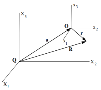
Consider the mass \({\alpha}\) at the location \(\mathbf{r} = (x_1, x_2, x_3)\) with respect to the origin of the center of mass body-fixed coordinate system \(O\). Transform to an arbitrary but parallel body-fixed coordinate system \(Q\), that is, the coordinate axes have the same orientation as the center of mass coordinate system. The location of the mass \({\alpha}\) with respect to this arbitrary coordinate system is \(\mathbf{R} = (X_1, X_2, X_3)\). That is, the general vectors for the two coordinates systems are related by

\[\mathbf{R} = \mathbf{a} + \mathbf{r} \label{13.34}\]

where \(\mathbf{a}\) is the vector connecting the origins of the coordinate systems \(O\) and \(Q\) illustrated in Figure \(\PageIndex{1}\). The elements of the inertia tensor with respect to axis system \(Q\), are given by equation \((13.4.1)\) to be

\[J_{i j} \equiv \sum_{\alpha}^{N} m_{\alpha}\left[\delta_{i j}\left(\sum_{k}^{3} X^2_{\alpha, k} \right) - X_{\alpha, i}X_{\alpha, j} \right] \]

The components along the three axes for each of the two coordinate systems are related by

\[X_i = a_i + x_i\]

Substituting these into the above inertia tensor relation gives

\[\begin{align}
J_{i j} &=\sum_{\alpha}^{N} m_{\alpha}\left[\delta_{i j}\left(\sum_{k}^{3}\left(x_{\alpha, k}+a_{i}\right)^{2}\right)-\left(x_{\alpha, i}+a_{i}\right)\left(x_{\alpha, j}+a_{i}\right)\right] \\
&=\sum_{\alpha}^{N} m_{\alpha}\left[\delta_{i j}\left(\sum_{k}^{3} x_{\alpha, k}^{2}\right)-x_{\alpha, i} x_{\alpha, j}\right]+\sum_{\alpha}^{N} m_{\alpha}\left[\delta_{i j}\left(\sum_{k}^{3}\left(2 x_{\alpha, k} a_{k}+a_{k}^{2}\right)\right)-\left(a_{i} x_{\alpha, j}+a_{j} x_{\alpha, i}+a_{i} a_{j}\right)\right]
\notag \end{align}\]

The first summation on the right-hand side corresponds to the elements \(I_{ij}\) of the inertia tensor in the center-of-mass frame. Thus the terms can be regrouped to give

\[J_{i j} \equiv I_{ij} + \sum_{\alpha}^{N} m_{\alpha} \left( \delta_{ij} \sum^3_k a^2_k - a_{i}a_j \right) + \sum_{\alpha}^{N} m_{\alpha}\left[2\delta_{i j} \sum_{k}^{3} x_{\alpha, k} a_{k} - a_i x_{\alpha, j} - a_{j} x_{\alpha, i} \right]\]

However, each term in the last bracket involves a sum of the form \(\sum^N_{\alpha} m_{\alpha} x_{\alpha ,k}\). Take the coordinate system \(O\) to be with respect to the center of mass for which

\[\sum^N_{\alpha} m_{\alpha} \mathbf{r}^{\prime} = 0 \]

This also applies to each component \(k\), that is

\[\sum^N_{\alpha} m_{\alpha} x_{\alpha ,k} = 0 \]

Therefore all of the terms in the last bracket cancel leaving

\[J_{i j} \equiv I_{ij} + \sum_{\alpha}^{N} m_{\alpha} \left( \delta_{ij} \sum^3_k a^2_k - a_{i}a_j \right)\]

But \(\sum^N_{\alpha} m_{\alpha} = M\) and \(\sum^3_k a^2_k = a^2\), thus

\[J_{ij} \equiv I_{ij} +M (a^2\delta_{ij} - a_ia_j)\]

where \(I_{ij}\) is the center-of-mass inertia tensor. This is the general form of Steiner’s parallel-axis theorem.

As an example, the moment of inertia around the \(X_1\) axis is given by

\[J_{11} \equiv I_{11} + M((a^2_1 + a^2_2 + a^3_3) \delta_{11} - a^2_1) = I_{11} + M(a^2_2 + a^2_3) \]

which corresponds to the elementary statement that the difference in the moments of inertia equals the mass of the body multiplied by the square of the distance between the parallel axes, \(x_1, X_1\). Note that the minimum moment of inertia of a body is \(I_{ij}\) which is about the center of mass.

Example \(\PageIndex{1}\): Inertia Tensor of a Solid Cube Rotating about the Center of Mass

The complicated expressions for the inertia tensor can be understood using the example of a uniform solid cube with side \(b\), density \(\rho\), and mass \(M = \rho b^3\), rotating about different axes. Assume that the origin of the coordinate system \(O\) is at the center of mass with the axes perpendicular to the centers of the faces of the cube.

Figure \(\PageIndex{2}\): Inertia tensor of a uniform solid cube of side \(b\) about the center of mass \(O\) and a corner of the cube \(Q\). The vector \(a\) is the vector distance between \(O\) and \(Q\).

The components of the inertia tensor can be calculated using \((13.4.2)\) written as an integral over the mass distribution rather than a summation.

\[I_{ij} = \int \rho ( \mathbf{r}^{\prime} ) \left(\delta_{ij} \left( \sum^3_k x^2_k \right) -x_ix_j\right) dV \nonumber\]

Thus

\[\begin{align*} I_{11} & = \rho \int^{b/2}_{-b/2} \int^{b/2}_{-b/2} \int^{b/2}_{-b/2} (x^2_2 + x^2_3) dx_3 dx_2 dx_1 \\[4pt] & = \frac{1}{6} \rho b^5 = \frac{1}{6} Mb^2 = I_{22} = I_{33} \end{align*}\]

By symmetry the diagonal moments of inertia about each face are identical. Similarly the products of inertia are given by

\[I_{12} = -\rho \int^{b/2}_{-b/2} \int^{b/2}_{-b/2} \int^{b/2}_{-b/2} (x_1x_2) dx_3 dx_2 dx_1 = 0\notag\]

Thus the inertia tensor is given by

\[\mathbf{I}^{cm} = \frac{1}{6} Mb^2 \begin{pmatrix} 1 & 0 & 0 \\ 0 & 1 & 0 \\ 0 & 0 & 1 \end{pmatrix} \notag\]

Note that this inertia tensor is diagonal implying that this is the principal axis system. In this case all three principal moments of inertia are identical and perpendicular to the centers of the faces of the cube. This is as expected from the symmetry of the cubic geometry.

Example \(\PageIndex{2}\): Inertia tensor of about a corner of a solid cube.

Direct calculation

Let one corner of the cube be the origin of the coordinate system \(Q\) and assume that the three adjacent sides of the cube lie along the coordinate axes. The components of the inertia tensor can be calculated using \((13.4.2)\). Thus

\[I_{11} = \rho \int^b_0 \int^b_0 \int^b_0 (x^2_2 + x^2_3) dx_3 dx_2 dx_1 = \frac{2}{3} \rho b^5 = \frac{2}{3} Mb^2 \notag\]

\[I_{12} = \rho \int^b_0 \int^b_0 \int^b_0 (x_1 x_2) dx_3 dx_2 dx_1 = -\frac{1}{4} \rho b^5 = - \frac{1}{4} Mb^2 \notag\]

Thus, evaluating all the nine components gives

\[\mathbf{I}^{corner} = \frac{1}{12} Mb^2 \begin{pmatrix} 8 & -3 & -3 \\ -3 & 8 & -3 \\ -3 & -3 & 8 \end{pmatrix} \nonumber\]

Parallel-axis theorem

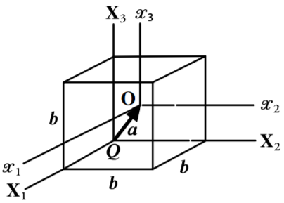
This inertia tensor also can be calculated using the parallel-axis theorem to relate the moment of inertia about the corner, to that at the center of mass. As shown in Figure \(\PageIndex{2}\), the vector \(a\) has components

\[a_1 = a_2 = a_3 = \frac{b}{2}\nonumber\]

Applying the parallel-axis theorem gives

\[J_{11} = I_{11} + M ( a^2 − a^2_1) = I_{11} + M ( a^2_2 + a^2_3) = \frac{1}{6} Mb^2 + \frac{1}{2} Mb^2 = \frac{2}{3} Mb^2 \nonumber\]

and similarly for \(J_{22}\) and \(J_{33}\). The off-diagonal terms are given by

\[J_{12} = I_{12} + M (−a_1a_2) = −\frac{1}{4}Mb^2 \nonumber\]

Thus the inertia tensor, transposed from the center of mass, to the corner of the cube is

\[\mathbf{I}^{corner} = \begin{pmatrix} \frac{2}{3} Mb^2 & -\frac{1}{4} Mb^2 & -\frac{1}{4} Mb^2 \\ -\frac{1}{4}Mb^2 & \frac{2}{3} Mb^2 & -\frac{1}{4} Mb^2\\ -\frac{1}{4} Mb^2 & -\frac{1}{4} Mb^2 & \frac{2}{3} Mb^2\end{pmatrix} = \frac{1}{12} Mb^2 \begin{pmatrix} 8 & -3 & -3 \\ -3 & 8 & -3 \\ -3 & -3 & 8 \end{pmatrix} \nonumber\]

This inertia tensor about the corner of the cube, is the same as that obtained by direct integration.

Principal moments of inertia

The coordinate axis frame used for rotation about the corner of the cube is not a principal axis frame. Therefore let us diagonalize the inertia tensor to find the principal axis frame and the principal moments of inertia about a corner. To achieve this requires solving the secular determinant

\[\begin{vmatrix} (\frac{2}{3} Mb^2 - I) & -\frac{1}{4} Mb^2 & -\frac{1}{4} Mb^2 \\ -\frac{1}{4} Mb^2 & (\frac{2}{3} Mb^2 - I) & -\frac{1}{4} Mb^2\\ -\frac{1}{4} Mb^2 & -\frac{1}{4} Mb^2 & (\frac{2}{3} Mb^2 - I) \end{vmatrix} = 0 \notag\]

The value of a determinant is not affected by adding or subtracting any row or column from any other row or column. Subtract row 1 from row 2 gives

\[\begin{vmatrix} (\frac{2}{3} Mb^2 - I) & -\frac{1}{4} Mb^2 & -\frac{1}{4} Mb^2 \\ -\frac{11}{12} Mb^2 & (\frac{11}{12} Mb^2 - I) & 0 \\ -\frac{1}{4} Mb^2 & -\frac{1}{4} Mb^2 & (\frac{2}{3} Mb^2 - I) \end{vmatrix} = 0 \notag\]

The determinant of this matrix is straightforward to evaluate and equals

\[\left(\frac{1}{6}Mb^2 - I \right) \left( \frac{11}{12}Mb^2 - I\right) \left(\frac{11}{12}Mb^2 - I \right) = 0 \nonumber\]

Thus the roots are

\[\mathbf{I}^{corner} = \begin{pmatrix} \frac{1}{6}Mb^2 & 0 & 0 \\ 0 & \frac{11}{12}Mb^2 & 0 \\ 0 & 0 & \frac{11}{12}Mb^2 \end{pmatrix}\notag\]

The identical roots \(I_{22} = I_{33} = \frac{11}{12} Mb^2\) imply that the principal axis associated with \(I_{11}\) must be a symmetry axis. The orientation can be found by substituting \(I_{11}\) into the above equation

\[(\{\mathbf{I}\} − I \{\mathbb{I}\}) \cdot \boldsymbol{\omega} = \frac{1}{12} Mb^2 \begin{pmatrix} 6 & −3 & −3\\ −3& 6 & −3\\ −3 &−3 & 6 \end{pmatrix} \begin{pmatrix} \omega_{11} \\ \omega_{21} \\ \omega_{31} \end{pmatrix} = 0 \notag\]

where the second subscript 1 attached to \(\omega_i\) signifies that this solution corresponds to \(I_{11}\). This gives

\[\begin{aligned} 2\omega_{11} − \omega_{21} − \omega_{31} = 0 \\ −\omega_{11} + 2\omega_{21} − \omega_{31} = 0 \\ −\omega_{11} − \omega_{21} + 2\omega_{31} = 0 \end{aligned}\]

Solving these three equations gives the unit vector for the first principal axis for which \(I_{11} = \frac{1}{6} Mb^2\) to be \(\mathbf{\hat{e}}_1= \frac{1}{\sqrt{3}} \begin{pmatrix} 1 \\ 1 \\ 1 \end{pmatrix}\). This can be repeated to find the other two principal axes by substituting \(I_{22} = \frac{11}{12} Mb^2\). This gives for the second principal moment \(I_{22}\)

\[(\{\mathbf{I}\} − I \{\mathbb{I}\}) \cdot \boldsymbol{\omega} = \frac{1}{12} Mb^2 \begin{pmatrix} −3 & −3 & −3\\ −3& −3& −3\\ −3 &−3 &−3 \end{pmatrix} \begin{pmatrix} \omega_{12} \\ \omega_{22} \\ \omega_{32} \end{pmatrix} = 0 \notag\]

This results in three identical equations for the components of \(\omega\) but all three equations are the same, namely

\[\omega_{12} + \omega_{22} + \omega_{32} = 0 \notag\]

This does not uniquely determine the direction of \(\omega\). However, it does imply that \(\omega_2\) corresponding to the second principal axis has the property that

\[\boldsymbol{\hat{\omega}} \cdot \mathbf{\hat{e}}_1 = 0 \notag\]

that is, any direction of \(\hat{e}_2\) that is perpendicular to \(\hat{e}_1\) is acceptable. In other words; any two orthogonal unit vectors \(\hat{e}_2\) and \(\hat{e}_3\) that are perpendicular to \(\hat{e}_1\) are acceptable. This ambiguity exists whenever two eigenvalues are equal; the three principal axes are only uniquely defined if all three eigenvalues are different. The same ambiguity exist when all three eigenvalues are identical as occurs for the principal moments of inertia about the center-of-mass of a uniform solid cube. This explains why the principal moment of inertia for the diagonal of the cube, that passes through the center of mass, has the same moment as when the principal axes pass through the center of the faces of the cube.