
14.8: Three-body coupled linear oscillator systems


- Last updated
- Jan 22, 2021
- Save as PDF

( \newcommand{\kernel}{\mathrm{null}\,}\)
Chapter 14.7 discussed parallel and series arrangements of two coupled oscillators. Extending from two to three coupled linear oscillators introduces interesting new characteristics of coupled oscillator systems. For more than two coupled oscillators, coupled oscillator systems separate into two classifications depending on whether each oscillator is coupled to the remaining n−1 oscillators, or when the coupling is only to the nearest neighbors as illustrated below.
Example 14.8.1: Three plane pendula; mean-field linear coupling
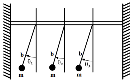
Consider three identical pendula with mass m and length b, suspended from a common support that yields slightly to pendulum motion leading to a coupling between all three pendula as illustrated in the adjacent figure. Assume that the motion of the three pendula all are in the same plane. This case is analogous to the piano where three strings in the treble section are coupled by the slightly-yielding common bridge plus sounding board leading to coupling between each of the three coupled oscillators. This case illustrates the important concept of degeneracy.
The generalized coordinates are the angles θ1, θ2, and θ3. Assume that the support yields such that the actual deflection angle for pendulum 1 is
θ′1=θ1−ε2(θ2+θ3)
where the coupling coefficient ε is small and involves all the pendula, not just the nearest neighbors. Assume that the same coupling relation exists for the other angle coordinates. The gravitational potential energy of each pendulum is given by
U1=mgb(1−cosθ1)≈12mgbθ21
assuming the small angle approximation. Ignoring terms of order ε2 gives that the potential energy
U=mgb2(θ′21+θ′22+θ′23)=mgb2(θ21+θ22+θ23−2εθ1θ2−2εθ1θ3−2εθ2θ3)
The kinetic energy evaluated at the equilibrium location is
T=12m(b˙θ1)2+12m(b˙θ2)2+12m(b˙θ3)2
The next stage is to evaluate the {T} and {V} tensors
T=mb2{100010001}V=mgb{1−ε−ε−ε1−ε−ε−ε1}
The third stage is to evaluate the secular determinant which can be written as
mgb|1−bgω2−ε−ε−ε1−bgω2−ε−ε−ε1−bgω2|=0
Expanding and factoring gives
(bgω2−1−ε)(bgω2−1−ε)(bgω2−1+2ε)=0
The roots are
ω1=√gb√1+εω2=√gb√1+εω3=√gb√1−2ε
This case results in two degenerate eigenfrequencies, ω1=ω2 while ω3 is the lowest eigenfrequency.
The eigenvectors can be determined by substitution of the eigenfrequencies into
n∑j(Vjk−ω2rTjk)ajr=0
Consider the lowest eigenfrequency ω3, i.e. r=3, for k=1, and substitute for ω3=√gb√1−2ε gives
2εa13−εa23−εa33=0
while for r=3, k=2
−εa13+2εa23−εa33=0
Solving these gives
a13=a23=a33
Assuming that the eigenfunction is normalized to unity
a213+a223+a233=1
then for the third eigenvector a3
a13=a23=a33=1√3
This solution corresponds to all three pendula oscillating in phase with the same amplitude, that is, a coherent oscillation.
Derivation of the eigenfunctions for the other two eigenfrequencies is complicated because of the degeneracy ω1=ω2, there are only five independent equations to specify the six unknowns for the eigenvectors a1 and a2. That is, the eigenvectors can be chosen freely as long as the orthogonality and normalization are satisfied. For example, setting a31=0, to remove the indeterminacy, results in the a matrix
{a}={12√216√613√3−12√216√613√30−13√613√3}
and thus the solution is given by
{θ1θ2θ3}={12√216√613√3−12√216√613√30−13√613√3}{η1η2η3}
The normal modes are obtained by taking the inverse matrix {a}−1 and using {η}={a}−1{θ}. Note that since {a} is real and orthogonal, then {a}−1 equals the transpose of {a}. That is;
{η1η2η3}={12√216√613√3−12√216√613√30−13√613√3}{θ1θ2θ3}
The normal mode η3 has eigenfrequency
ω3=√gb√1−2ε
and eigenvector
η3=1√3(θ1,θ2,θ3)
This corresponds to the in-phase oscillation of all three pendula.
The other two degenerate solutions are
η1=1√2(θ1,−θ2,0)η2=1√6(θ1,θ2,−2θ3)
with eigenvalues
ω1=ω2=√gb√1+ε
These two degenerate normal modes correspond to two pendula oscillating out of phase with the same amplitude, or two oscillating in phase with the same amplitude and the third out of phase with twice the amplitude. An important result of this toy model is that the most symmetric mode η3 is pushed far from all the other modes. Note that for this example, the coherent mode a3 corresponds to the center-of-mass oscillation with no relative motion between the three pendula. This is in contrast to the eigenvectors a1 and a2 which both correspond to relative motion of the pendula such that there is zero center-of-mass motion. This mean-field coupling behavior is exhibited by collective motion in nuclei as discussed in example 14.12.1.
Example 14.8.2: Three plane pendula; nearest-neighbor coupling
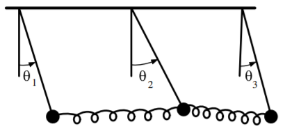
There is a large and important class of coupled oscillators where the coupling is only between nearest neighbors; a crystalline lattice is a classic example. A toy model for such a system is the case of three identical pendula coupled by two identical springs, where only the nearest neighbors are coupled as shown in the adjacent figure. Assume the identical pendula are of length b and mass m. As in the last example, the kinetic energy evaluated at the equilibrium location is
T=12mb2˙θ21+12mb2˙θ22+12mb2˙θ23
The gravitational potential energy of each pendulum equals mgb(1−cosθ)≈12mgbθ2 thus
Ugrav=12mgb(θ21+θ22+θ23)
while the potential energy in the springs is given by
Uspring=12κb2[(θ2−θ1)2+(θ3−θ2)2]=12κb2[θ21+2θ22+θ23−2θ1θ2−2θ2θ3]
Thus the total potential energy is given by
U=12mgb(θ21+θ22+θ23)+12κb2[θ21+2θ22+θ23−2θ1θ2−2θ2θ3]
The Lagrangian then becomes
L=12mb2(˙θ21+˙θ22+˙θ23)−12(mgb+κb2)θ21+12(mgb+2κb2)θ22+12(mgb+κb2)θ23−κb2(θ1θ2+θ2θ3)
Using this in the Euler-Lagrange equations gives the equations of motion
mb2¨θ1−(mgb+κb2)θ1+κb2θ2=0mb2¨θ2−(mgb+2κb2)θ2+κb2(θ1+θ3)=0mb2¨θ3−(mgb+κb2)θ3+κb2θ2=0
The general analytic approach requires the T and V energy tensors given by
T=mb2{100010001}V={mgb+κb2−κb20−κb2mgb+2κb2−κb20−κb2mgb+κb2}
Note that in contrast to the prior case of three fully-coupled pendula, for the nearest neighbor case the potential energy tensor {V} is non-zero only on the diagonal and ±1 components parallel to the diagonal.
The third stage is to evaluate the secular determinant of the (V−ω2T) matrix, that is
|mgb+κb2−ω2mb2−κb20−κb2mgb+2κb2−ω2mb2−κb20−κb2mgb+κb2−ω2mb2|=0
This results in the characteristic equation
(mgb−ω2mb2)(mgb+κb2−ω2mb2)(mgb+3κb2−ω2mb2)=0
which results in the three non-degenerate eigenfrequencies for the normal modes.
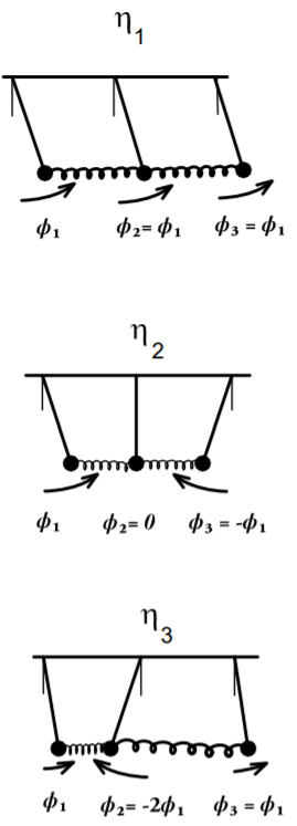
The normal modes are similar to the prior case of complete linear coupling, as shown in the adjacent figure.
ω1=√gb This lowest mode η1 involves the three pendula oscillating in phase such that the springs are not stretched or compressed thus the period of this coherent oscillation is the same as an independent pendulum of mass m and length b. That is
η1=1√3(θ1,θ2,θ3)
ω2=√gb+κm. This second mode η2 has the central mass stationary with the outer pendula oscillating with the same amplitude and out of phase. That is
η2=1√2(θ1,0,−θ3)
ω3=√gb+3κm. This third mode η3 involves the outer pendula in phase with the same amplitude while the central pendulum oscillating with angle θ3=−2θ1. That is
η3=1√6(θ1,−2θ2,θ3)
Similar to the prior case of three completely-coupled pendula, the coherent normal mode η1 corresponds to an oscillation of the center-of-mass with no relative motion, while η2 and η3 correspond to relative motion of the pendula with stationary center of mass motion. In contrast to the prior example of complete coupling, for nearest neighbor coupling the two higher lying solutions are not degenerate. That is, the nearest neighbor coupling solutions differ from when all masses are linearly coupled.
It is interesting to note that this example combines two coupling mechanisms that can be used to predict the solutions for two extreme cases by switching off one of these coupling mechanisms. Switching off the coupling springs, by setting κ=0, makes all three normal frequencies degenerate with ω1=ω2=ω3=√gb. This corresponds to three independent identical pendula each with frequency ω=√gb. Also the three linear combinations η1,η2,η3 also have this same frequency, in particular η1 corresponds to an in-phase oscillation of the three pendula. The three uncoupled pendula are independent and any combination the three modes is allowed since the three frequencies are degenerate.
The other extreme is to let gb=0, that is switch off the gravitational field or let b→∞, then the only coupling is due to the two springs. This results in ω1=0 because there is no restoring force acting on the coherent motion of the three in-phase coupled oscillators; as a result, oscillatory motion cannot be sustained since it corresponds to the center of mass oscillation with no external forces acting which is spurious. That is, this spurious solution corresponds to constant linear translation.
Example 14.8.3: System of three bodies coupled by six springs
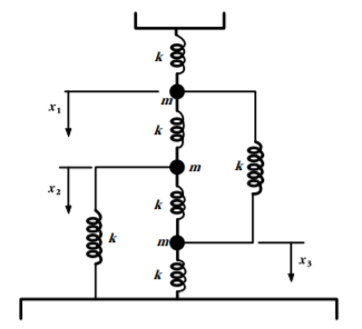
Consider the completely-coupled mechanical system shown in the adjacent figure.
1) The first stage is to determine the potential and kinetic energies using an appropriate set of generalized coordinates, which here are x1 and x2. The potential energy is the sum of the potential energies for each of the six springs
U=32κx21+32κx22+32κx23−κx1x2−κx1x3−κx2x3
while the kinetic energy is given by
T=12m˙x21+12m˙x22+12m˙x23
2) The second stage is to evaluate the potential energy V and kinetic energy T tensors.
V={3κ−κ−κ−κ3κ−κ−κ−κ3κ}T={M000M000M}
Note that for this case the kinetic energy tensor is diagonal whereas the potential energy tensor is nondiagonal and corresponds to complete coupling of the three coordinates.
3) The third stage is to use the potential V and kinetic T energy tensors to evaluate the secular determinant giving
|(3κ−mω2)−κ−κ−κ(3κ−mω2)−κ−κ−κ(3κ−mω2)|=0
The expansion of this secular determinant yields
(κ−mω2)(4κ−mω2)(4κ−mMω2)=0
The solution for this complete-coupled system has two degenerate eigenvalues.
ω1=ω2=2√κmω3=√κm
4) The fourth step is to insert these eigenfrequencies into the secular equation
∑j(Vjk−ω2rTjk)ajr=0
to determine the coefficients ajr.
5) The final stage is to write the general coordinates in terms of the normal coordinates.
The result is that the angular frequency ω3=√κm corresponds to a normal mode for which the three masses oscillate in phase corresponding to a center-of-mass oscillation with no relative motion of the masses.
η3=1√3(x1+x2+x3)
For this coherent motion only one spring per mass is stretched resulting in the same frequency as one mass on a spring. The other two solutions correspond to the three masses oscillating out of phase which implies all three springs are stretched and thus the angular frequency is higher. Since the two eigenvalues ω1=ω2=2√κm are degenerate then there are only five independent equations to specify the six unknowns for the degenerate eigenvalues. Thus it is possible to select a combination of the eigenvectors η1 and η2 such that the combination is orthogonal to η3. Choose a31=0 to removes the indeterminacy. Then adding or subtracting gives that the normal modes are
η1=1√2(x1−x2+0)η2=1√2(x1+x2−2x3)
These two degenerate normal modes correspond to relative motion of the masses with stationary center-of-mass.