
15.5: Action-angle Variables


- Last updated
- Mar 14, 2021
- Save as PDF

( \newcommand{\kernel}{\mathrm{null}\,}\)
Canonical transformation
Systems possessing periodic solutions are a ubiquitous feature in physics. The periodic motion can be either an oscillation, for which the trajectory in phase space is a closed loop (libration), or rolling (rotational) motion as discussed in chapter 3.4. For many problems involving periodic motion, the interest often lies in the frequencies of motion rather than the detailed shape of the trajectories in phase space. The action-angle variable approach uses a canonical transformation to action and angle variables which provide a powerful, and elegant method to exploit Hamiltonian mechanics. In particular, it can determine the frequencies of periodic motion without having to calculate the exact trajectories for the motion. This method was introduced by the French astronomer Ch. E. Delaunay(1816 − 1872) for applications to orbits in celestial mechanics, but it has equally important applications beyond celestial mechanics such as to bound solutions of the atom in quantum mechanics.
The action-angle method replaces the momenta in the Hamilton-Jacobi procedure by the action phase integral for the closed loop (libration) trajectory in phase space defined by
Ji≡∮pidqi
where for each cyclic variable the integral is taken over one complete period of oscillation. The cyclic variable Ii is called the action variable where
Ii≡12πJi=12π∮pidqi
The canonical variable to the action variable I is the angle variable ϕ. Note that the name “action variable” is used to differentiate I from the action functional S=∫Ldt which has the same units; i.e. angular momentum.
The general principle underlying the use of action-angle variables is illustrated by considering one body, of mass m, subject to a one-dimensional bound conservative potential energy U(q). The Hamiltonian is given by
H(p,q)=p22m+U(q)
This bound system has a (q,p) phase space contour for each energy H=E.
p(q,E)=±√2m(E−U(q))
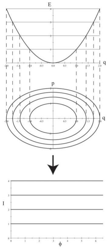
For an oscillatory system the two-valued momentum of Equation ??? is non-trivial to handle. By contrast, the area J≡∮pdq of the closed loop in phase space is a single-valued scalar quantity that depends on E and U(q). Moreover, Liouville’s theorem states that the area of the closed contour in phase space J≡∮pdq is invariant to canonical transformations. These facts suggest the use of a new pair of conjugate variables, (ϕ,I), where I(E) uniquely labels the trajectory, and corresponding area, of a closed loop in phase space for each value of E, and the single-valued function ϕ is a corresponding angle that specifies the exact point along the phase-space contour as illustrated in Fig 15.5.1.
For simplicity consider the linear harmonic oscillator where
U(q)=12mω2q2
Then the Hamiltonian, ??? equals
H(p,q)=p22m+12mω2q2
Hamilton’s equations of motion give that
˙p=−∂H∂q=−mω2q
˙q=∂H∂p=pm
The solution of equations ??? and ??? is of the form
q=Ccos(ω(t−t0))
p=−mωCsinω(t−t0)
where C, and t0 are integration constants. For the harmonic oscillator, equations ??? and ??? correspond to the usual elliptical contours in phase space, as illustrated in Figure 15.5.1.
The action-angle canonical transformation involves making the transform
(q,p)→(ϕ,I)
where I is defined by Equation ??? and the angle ϕ being the corresponding canonical angle. The logical approach to this canonical transformation for the harmonic oscillator is to define q and p in terms of ϕ and I
q=√2Imωcosϕ
p=√2mIωsinϕ
Note that the Poisson bracket is unity
[q,p](ϕ,I)=1
which implies that the above transformation is canonical, and thus the phase space area I(E)≡12π∮pdq is conserved.
For this canonical transformation the transformed Hamiltonian H(ϕ,I) is
H(ϕ,I)=12m(2mωI)sin2ϕ+12mω22Imωcos2ϕ=ωI
Note that this Hamiltonian is a constant that is independent of the angle ϕ, and thus Hamilton’s equations of motion give
˙I=−∂H(ϕ,I)∂ϕ=0
˙ϕ=∂H(ϕ,I)∂I=ω
Thus we have mapped the harmonic oscillator to new coordinates (ϕ,I) where
I=H(ϕ,I)ω=Eω
ϕ=ω(t−t0)
That is, the phase space has been mapped from ellipses, with area proportional to E in the (q,p) phase space, to a cylindrical (ϕ,I) phase space where I=Eω are constant values that are independent of the angle, while ϕ increases linearly with time. Thus the variables (q,p) are periodic with modulus Δϕ=2π.
q(ϕ+2π,I)=q(ϕ,I)
p(ϕ+2π,I)=p(ϕ,I)
The period τ of the periodic oscillatory motion is given simply by Δϕ=2π=ωτ which is the well known result for the harmonic oscillator. Note that the action-angle variable canonical transformation has determined the frequency of the periodic motion without solving the detailed trajectory of the motion.
The above example of the harmonic oscillator has shown that, for integrable periodic systems, it is possible to identify a canonical transformation to (ϕ,I) such that the Hamiltonian is independent of the angle ϕ which specifies the instantaneous location on the constant energy contour I. If the phase space contour is a separatrix, then it divides phase space into invariant regions containing phase-space contours with differing behavior. The action-angle variables are not useful for separatrix contours. For rolling motion, the system rotates with continuously increasing, or decreasing angle, and there is no natural boundary for the action angle variable since the phase space trajectory is continuous and not closed. However, the action-angle approach still is valid if the motion involves periodic as well as rolling motion.
The example of the one-dimensional, one-body, harmonic oscillator can be expanded to the more general case for many bodies in three dimensions. This is illustrated by considering multiple periodic systems for which the Hamiltonian is conservative and where the equations of the canonical transformation are separable. The generalized momenta then can be written as
pi=∂Wi(qi;α1,α2,..αn)∂qi
for which each pi is a function of qi and the n integration constants αj
pi=pi(qi,α1,α2,..αn)
The momentum pi(qi,α1,α2,..αn) represents the trajectory of the system in the (qi,pi) phase space that is characterized by Hamilton’s characteristic function W(q,J). Combining equations ???, ??? gives
Ji≡∮∂Wi(qi;α1,α2,..αn)∂qidqi
Since qi is merely a variable of integration, each active action variable Ji is a function of the n constants of integration in the Hamilton-Jacobi equation. Because of the independence of the separable-variable pairs (qi,pi), the Ji form n independent functions of the αi, and hence are suitable for use as a new set of constant momenta. Thus the characteristic function W can be written as
W(q1,...qn;J1,...Jn)=∑jWj(qj;J1,...Jn)
while the Hamiltonian is only a function of the momenta H(J1,....Jn)
The generalized coordinate, conjugate to J, is known as the angle variable ϕi which is defined by the transformation equation
ϕi=∂W∂Ji=n∑j=1∂Wj(qj;J1,...Jn)∂Ji
The corresponding equation of motion for ϕ is given by
˙ϕi=∂H(J)∂Ji=2πωi(J1,...Jn)
where ωi(J) are constant functions of the action variables Jj with a solution
ϕi=2πωit+βi
that is, they are linear functions of time. The constants ωi can be identified with the frequencies of the multiple periodic motions.
The action-angle variables appear to be no different than a particular set of transformed coordinates. Their merit appears when the physical interpretation is assigned to ωi. Consider the change δϕi as the qj are changed infinitesimally
δϕi=∑j∂ϕi∂qj∂qj=∑j∂2W∂Ji∂qj∂qj
The derivative with respect to qi vanishes except for the Wj component of W. Thus Equation ??? reduces to
δϕi=∂∂Ji∑jpj(qj,J)dqj
Therefore, the total change in ϕ, as the system goes through one complete cycle is
Δϕi=∑j∂∂Ji∮pj(qj,J)dqj=2πδij
where ∂∂Ji is outside the integral since the Ji are constants for cyclic motion. Thus Δϕi=2π=ωiτi where τi is the period for one cycle of oscillation, where the angular frequency ωi is given by
ωi2π=νi=1τi
Thus the frequency ν associated with the periodic motion is the reciprocal of the period τ. The secret here is that the derivative of H with respect to the action variable J given by Equation ??? directly determines the frequency of the periodic motion without the need to solve the complete equations of motion. Note that multiple periodic motion can be represented by a Fourier expansion of the form
qk=∞∑j1=−∞∞∑j2=−∞...∞∑jn=−∞akj1,..,jne2πi(j1ω1+j2ω2+j3ω3+..+jnωn)
Although the action-angle approach to Hamilton-Jacobi theory does not produce complete equations of motion, it does provide the frequency decomposition that often is the physics of interest. The reason that the powerful action-angle variable approach has been introduced here is that it is used extensively in celestial mechanics. The action-angle concept also played a key role in the development of quantum mechanics, in that Sommerfeld recognized that Bohr’s ad hoc assumption that angular momentum is quantized, could be expressed in terms of quantization of the angle variable as is mentioned in chapter 18.
Adiabatic invariance of the action variables
When the Hamiltonian depends on time it can be quite difficult to solve for the motion because it is difficult to find constants of motion for time-dependent systems. However, if the time dependence is sufficiently slow, that is, if the motion is adiabatic, then there exist dynamical variables that are almost constant which can be used to solve for the motion. In particular, such approximate constants are the familiar action-angle integrals. The adiabatic invariance of the action variables played an important role in the development of quantum mechanics during the 1911 Solvay Conference. This was a time when physicists were grappling with the concepts of quantum mechanics. Einstein used the following classical mechanics example of adiabatic invariance, applied to the simple pendulum, in order to illustrate the concept of adiabatic invariance of the action. This example demonstrates the power of using action-angle variables.
Example 15.5.1: Adiabatic invariance for the simple pendulum
Consider that the pendulum is made up of a point mass M suspended from a pivot by a light string of length L that is swinging freely in a vertical plane. Derive the dependence of the amplitude of the oscillations θ, assuming θ is small, if the string is very slowly shortened by a factor of 2, that is, assume that the change in length during one period of the oscillation is very small. The tension in the string T is given by
T=Mg⟨cosθ⟩+⟨ML2˙θ2L⟩
Let the pendulum angle be oscillatory
θ=θ0cos(ωt+φ0)
Then the average mean square amplitude and velocity over one period are
⟨θ2⟩=⟨[θ0cos(ωt+φ0)]2⟩=θ202
⟨˙θ2⟩=⟨[−θ0ωsin(ωt+φ0)]2⟩=ω2θ202
Since, for the simple pendulum, ω2=gL, then the tension in the string
T=Mg(1−⟨θ2⟩2)+ML⟨˙θ2⟩=Mg(1+θ204)
Assuming that θ0 is a small angle, and that the change in length −ΔL is very small during one period τ, then the work done is
ΔW=TΔL=−MgΔL−Mgθ204ΔL
while the change in internal oscillator energy is
Δ(−MgLcosθ0)=Δ[−MgL(1−θ202)]=−MgΔL+12MgΔ(Lθ20)=−MgΔL+12Mgθ20ΔL+MgLθ0Δθ0
The work done must balance the increment in internal energy therefore
Lθ0Δθ0+3θ20ΔL4=0
or
Lθ20Δln(θ0L34)=0
Therefore it follows that
(θ0L34)= constant
or
θ0∝L−34
Thus shortening the length of the pendulum string from L to L2 adiabatically corresponds to the amplitude increasing by a factor 1.68.
Consider the action-angle integral for one closed period τ=2πω for this problem
J=∮Pθdθ=∮ML2˙θ⋅˙θdt=ML2⟨˙θ2⟩2πω=πML2θ20ω=πMg12θ20L32= constant
where that last step is due to Equation c.
The above example shows that the action integral J=constant, that is, it is invariant to an adiabatic change. In retrospect this result is as expected in that the action integral should be minimized.