
15.4: Hamilton-Jacobi Theory


- Last updated
- Jun 28, 2021
- Save as PDF

( \newcommand{\kernel}{\mathrm{null}\,}\)
Hamilton used the Principle of Least Action to derive the Hamilton-Jacobi relation (chapter 15.3)
H(q,p,t)+∂S∂t=0
where q,p refer to the 1≤i≤n variables qi,pi and S(qj(t1),t1,qj(t2),t2) is the action functional. Integration of this first-order partial differential equation is non trivial which is a major handicap for practical exploitation of the Hamilton-Jacobi equation. This stimulated Jacobi to develop the mathematical framework for canonical transformation that are required to solve the Hamilton-Jacobi equation. Jacobi’s approach is to exploit generating functions for making a canonical transformation to a new Hamiltonian H(Q,P,t) that equals zero.
H(Q,P,t)=H(q,p,t)+∂S∂t=0
The generating function for solving the Hamilton-Jacobi equation then equals the action functional S.
The Hamilton-Jacobi theory is based on selecting a canonical transformation to new coordinates (Q,P,t) all of which are either constant, or the Qi are cyclic, which implies that the corresponding momenta Pi are constants. In either case, a solution to the equations of motion is obtained. A remarkable feature of Hamilton-Jacobi theory is that the canonical transformation is completely characterized by a single generating function, S. The canonical equations likewise are characterized by a single Hamiltonian function, H. Moreover, the generating function S, and Hamiltonian function H, are linked together by Equation ???. The underlying goal of Hamilton-Jacobi theory is to transform the Hamiltonian to a known form such that the canonical equations become directly integrable. Since this transformation depends on a single scalar function, the problem is reduced to solving a single partial differential equation.
Time-dependent Hamiltonian
Jacobi’s complete integral S(qi,Pi,t)
The principle underlying Jacobi’s approach to Hamilton-Jacobi theory is to provide a recipe for finding the generating function F=S needed to transform the Hamiltonian H(q,p,t) to the new Hamiltonian H(Q,P,t) using Equation ???. When the derivatives of the transformed Hamiltonian H(Q,P,t) are zero, then the equations of motion become
˙Qi=∂H∂Pi=0
˙Pi=−∂H∂Qi=0
and thus Qi and Pi are constants of motion. The new Hamiltonian H must be related to the original Hamiltonian H by a canonical transformation for which
H(Q,P,t)=H(q,p,t)+∂S∂t
Equations ??? and ??? are automatically satisfied if the new Hamiltonian H=0 since then Equation ??? gives that the generating function S satisfies Equation ???.
Any of the four types of generating function can be used. Jacobi chose the type 2 generating function as being the most useful for many practical cases, that is, S(qi,Pi,t) which is called Jacobi’s complete integral.
For generating functions F1 and F2 the generalized momenta are derived from the action by the derivative
pi=∂S∂qi
Use this generalized momentum to replace pi in the Hamiltonian H, given in Equation ???, leads to the Hamilton-Jacobi equation expressed in terms of the action S.
H(q1,...qn;∂S∂q1,...,∂S∂qn;t)+∂S∂t=0
The Hamilton-Jacobi equation, ???, can be written more compactly using tensors q and ∇S to designate (q1,..qn) and ∂S∂q1,...,∂S∂qn respectively. That is
H(q,∇S,t)+∂S∂t=0
Equation ??? is a first-order partial differential equation in n+1 variables which are the old spatial coordinates qi plus time t. The new momenta Pi have not been specified except that they are constants since H=0.
Assume the existence of a solution of ??? of the form S(qi,Pi,t)=S(q1,..qn;α1,..αn+1;t) where the generalized momenta Pi=α1,α2,....α plus t are the n+1 independent constants of integration in the transformed frame. One constant of integration is irrelevant to the solution since only partial derivatives of S(qi,Pi,t) with respect to qi and t are involved. Thus, if S is a solution of the first-order partial differential equation, then so is S+α where α is a constant. Thus it can be assumed that one of the n+1 constants of integration is just an additive constant which can be ignored leading effectively to a solution
S(qi,Pi,t)=S(q1,.....qn;α1,.....αn;t)
where none of the n independent constants are solely additive. Such generating function solutions are called complete solutions of the first-order partial differential equations since all constants of integration are known.
It is possible to assume that the n generalized momenta, Pi are constants αi, where the αi are the constants. This allows the generalized momentum to be written as
pi=∂S(q,α,t)∂qi
Similarly, Hamilton’s equations of motion give the conjugate coordinate Q=β, where βi are constants. That is
Qi=βi=∂S(q,α,t)∂αi
The above procedure has determined the complete set of 2n constants (Q=β,P=α). It is possible to invert the canonical transformation to express the above solution, which is expressed in terms of Qi=βi and Pi=αi, back to the original coordinates, that is, qj=qj(α,β,t) and momenta pj=pj(α,β,t) which is the required solution.
Hamilton’s principle function SH(qi,t;qoto)
Hamilton’s approach to solving the Hamilton-Jacobi Equation ??? is to seek a canonical transformation from variables (p,q) at time t, to a new set of constant quantities, which may be the initial values (q0,p0) at time t=0. Hamilton’s principle function SH(qi,t;qoto) is the generating function for this canonical transformation from the variables (q,p) at time t to the initial variables (q0,p0) at time t0. Hamilton’s principle function SH(qi,t;qoto) is directly related to Jacobi’s complete integral S(qi,Pi,t).
Note that SH is the generating function of a canonical transformation from the present time (q,p,t) variables to the initial (q0,p0,t0), whereas Jacobi’s S is the generating function of a canonical transformation from the present (q,p,t) variables to the constant variables (Q=β,P=α). For the Hamilton approach, the canonical transformation can be accomplished in two steps using S by first transforming from (q,p,t) at time t, to (β,α), then transforming from (β,α) to (q0,p0,t0). That is, this two-step process corresponds to
SH(q,t;qoto)=S(q,α,t)−S(q0,α,t0)
Hamilton’s principle function SH(q,t;qoto) is related to Jacobi’s complete integral S(q,α,t), and it will not be discussed further in this book.
Time-independent Hamiltonian
Frequently the Hamiltonian does not explicitly depend on time. For the standard Lagrangian with time-independent constraints and transformation, then H(q,p,t)=E which is the total energy. For this case, the Hamilton-Jacobi equation simplifies to give
∂S∂t=−H(q,p,t)=−E(α)
The integration of the time dependence is trivial, and thus the action integral for a time-independent Hamiltonian equals
S(q,α,t)=W(q,α)−E(α)t
That is, the action integral has separated into a time independent term W(q,α) which is called Hamilton’s characteristic function plus a time-dependent term −E(α)t. Thus using equations ???, ??? gives that the generalized momentum is
pi=∂W(q,α)∂qi
The physical significance of Hamilton’s characteristic function W(q,α) can be understood by taking the total time derivative
dWdt=∑i∂W(q,α)∂qi˙qi=∑ipi˙qi
Taking the time integral then gives
W(q,α)=∫∑pi˙qidt=∫∑pidqi
Note that this equals the abbreviated action described in chapter 9.2.3, that is W(q,α)=S0(q,α).
Inserting the action S(q,α) into the Hamilton-Jacobi equation (15.2.1) gives
H(q;∂W(q,α)∂q)=E(α)
This is called the time-independent Hamilton-Jacobi equation. Usually it is convenient to have E equal the total energy. However, sometimes it is more convenient to exclude the kth energy E(αk) in the set, in which case E=E(α1,α2,...αk−1); the Routhian exploits this feature.
The equations of the canonical transformation expressed in terms of W(q,α) are
pi=∂W(q,α)∂qiβi+∂E(α)∂αit=∂W(q,α)∂αi
These equations show that Hamilton’s characteristic function W(q,α) is itself the generating function of a time-independent canonical transformation from the old variables (q,p) to a set of new variables
Qi=βi+∂E(α)∂αitPi=αi
Table 15.4.1 summarizes the time-dependent and time-independent forms of the Hamilton-Jacobi equation.
| Hamiltonian | Time dependent H(q,p,t) | Time independent H(q,p) |
| Transformed Hamiltonian | H=0 | H is cyclic |
| Canonical transformed variables | All QiPi are constants of motion | All Pi are constants of motion |
| Transformed equations of motion |
˙Qi=∂H∂Pi=0, therefore Qi=βi ˙Pi=−∂H∂Qi=0, therefore Pi=αi |
˙Qi=∂H∂Pi=vi, therefore Qi=vit+βi ˙Pi=−∂H∂Qi=0, therefore Pi=αi |
| Generating function | Jacobi’s complete integral S(q,P,t) | Characteristic Function W(q,P) |
| Hamilton-Jacobi equation | H(q1,...qn;∂S∂q1,...,∂S∂qn;t)+∂S∂t=0 | H(q1,...qn;∂W∂q1,...,∂W∂qn)=E |
| Transformation equations |
pi=∂S∂qi Qi=∂S∂αi=βi |
pi=∂W∂qi Qi=∂W∂αi=vit+βi |
Separation of variables
Exploitation of the Hamilton-Jacobi theory requires finding a suitable action function S. When the Hamiltonian is time independent, then Equation ??? shows that the time dependence of the action integral separates out from the dependence on the spatial variables. For many systems, the Hamilton’s characteristic function W(q,P) separates into a simple sum of terms each of which is a function of a single variable. That is,
W(q,α)=W1(q1)+W2(q2)+⋯⋅⋅Wn(qn)
where each function in the summation on the right depends only on a single variable. Then Equation ??? reduces to
H(q1,...qn;∂W∂q1,...,∂W∂qn)=E
where E is the constant denoting the total energy.
Hamilton’s characteristic function W(q,P) can be used with equations ???, ???, ???, ???, and ??? to derive
pi=∂W(q,α)∂qiQi=∂W(q,α)∂Pi
˙Qi=∂H∂Pi=0˙Pi=∂H∂Qi=0
H=H+∂S∂t=H−E=0
which has reduced the problem to a simple sum of one-dimensional first-order differential equations.
If the ith variable is cyclic, then the Hamiltonian is not a function of qi and the ith term in Hamilton’s characteristic function equals Wi=αiqi which separates out from the summation in Equation ???. That is, all cyclic variables can be factored out of W(q,α) which greatly simplifies solution of the Hamilton-Jacobi equation. As a consequence, the ability of the Hamilton-Jacobi method to make a canonical transformation to separate the system into many cyclic or independent variables, which can be solved trivially, is a remarkably powerful way for solving the equations of motion in Hamiltonian mechanics.
Example 15.4.1: Free particle
Consider the motion of a free particle of mass m in a force-free region. Then Equation ??? reduces to
H(q1,...qn;∂S∂q1,...,∂S∂qn;t)+∂S∂t=0
Since no forces act, and the momentum p=∇S, thus the Hamilton-Jacobi equation reduces to
12m∇2S+∂S∂t=0
The Hamiltonian is time independent, thus Equation ??? applies
S(q,t)=W(q,α)−E(α)t
Since the Hamiltonian does not explicitly depend on the coordinates (x,y,z), then the coordinates are cyclic and separation of the variables, ???, gives that the action
S=α⋅r−Et
For Equation B to be a solution of Equation A requires that
E=12mα2
Therefore
S=α⋅r−12mα2t
Since
˙Q=∂S∂α=r−αmt
the equation of motion and the conjugate momentum are given by
r=˙Q+αmtp=∇S=α
Thus the Hamilton-Jacobi relation has given both the equation of motion and the linear momentum p.
Example 15.4.2: Point particle in a uniform gravitational field
The Hamiltonian is
H=12m(p2x+p2y+p2z)+mgz
Since the system is conservative, then the Hamilton-Jacobi equation can be written in terms of Hamilton’s characteristic function W
E=12m[(∂W∂x)2+(∂W∂y)2+(∂W∂z)2]+mgz
Assuming that the variables can be separated W=X(x)+Y(y)+Z(z) leads to
px=∂X(x)∂x=αx
py=∂Y(y)∂y=αy
pz=∂Z(z)∂z=√2m(E−mgz)−α2x−α2y
Thus by integration the total W equals
W=∫xx0αxdx+∫yy0αydy+∫zz0(√2m(E−mgz)−α2x−α2y)dz
Therefore using ??? gives
βz=t−t0=∫zz0mdz√2m(E−mgz)−α2x−α2y
βx= constant =(x−x0)−∫zz0αxdz√2m(E−mgz)−α2x−α2y
βy= constant =(y−y0)−∫zz0αydz√2m(E−mgz)−α2x−α2y
If x0,y0,z0 is the position of the particle at time t=t0 then βx=βy=0, and from ???
x−x0=(αxm)(t−t0)
y−y0=(αym)(t−t0)
z−z0=(√2m(E−mgz)−α2x−α2ym)(t−t0)−12g(t−t0)2
This corresponds to a parabola as should be expected for this trivial example.
Example 15.4.3: One-dimensional harmonic oscillator
As discussed in example 15.3.5 the Hamiltonian for the one-dimensional harmonic oscillator can be written as
H=12m(p2+m2ω2q2)=E
assuming it is conservative and where ω=√km.
Hamilton’s characteristic function W can be used where
S(q,E,t)=W(q,E)−Et
pi=∂W∂qi
Inserting the generalized momentum pi into the Hamiltonian gives
12m([∂W∂q]2+m2ω2q2)=E
Integration of this equation gives
W=√2mE∫dq√1−mω2q22E
That is
S=√2mE∫dq√1−mω2q22E−Et
Note that
∂S(q,E,t)∂E=√2mE∫dq√1−mω2q22E−t
This can be integrated to give
t=1ωarcsin(q√mω22E)+t0
That is
q=√2Emω2sinω(t−t0)
This is the familiar solution of the undamped harmonic oscillator.
Example 15.4.4: The central force problem
The problem of a particle acted upon by a central force occurs frequently in physics. Consider the mass m acted upon by a time-independent central potential energy U(r). The Hamiltonian is time independent and can be written in spherical coordinates as
H=12m(p2r+1r2p2θ+1r2sin2θp2ψ)+U(r)=E
The time-independent Hamilton-Jacobi equation is conservative, thus
12m[(∂W∂r)2+1r2(∂W∂θ)2+1r2sin2θ(∂W∂ϕ)2]+U(r)=E
Try a separable solution for Hamilton’s characteristic function W of the form
W=R(r)+Θ(θ)+Φ(ϕ)
The Hamilton-Jacobi equation then becomes
12m[(∂R∂r)2+1r2(∂Θ∂θ)2+1r2sin2θ(∂Φ∂ϕ)2]+U(r)=E
This can be rearranged into the form
2mr2sin2θ{12m[(∂R∂r)2+1r2(∂Θ∂θ)2]+U(r)+E}=−(∂Φ∂ϕ)2
The left-hand side is independent of ϕ whereas the right-hand side is independent of r and θ. Both sides must equal a constant which is set to equal −L2z, that is
12m[(∂R∂r)2+1r2(∂Θ∂θ)2]+U(r)+L2z2mr2sin2θ=E
(∂Φ∂ϕ)2=L2z
The equation in r and θ can be rearranged in the form
2mr2[12m(∂R∂r)2+U(r)−E]=−[(∂Θ∂θ)2+L2zsin2θ]
The left-hand side is independent of θ and the right-hand side is independent of r so both must equal a constant which is set to be −L2
12m(∂R∂r)2+U(r)+L22mr2=E
(∂Θ∂θ)2+L2zsin2θ=L2
The variables now are completely separated and, by rearrangement plus integration, one obtains
R(r)=√2m∫√E−U(r)−L22mr2dr
Θ(θ)=∫√L2−L2zsin2θdθ
Φ(ϕ)=Lzϕ
Substituting these into W=R(r)+Θ(θ)+Φ(ϕ) gives
W=√2m∫√E−U(r)−L22mr2dr+∫√L2−L2zsin2θdθ+Lzϕ
Hamilton’s characteristic function W is the generating function from coordinates (r,θ,ϕ,pr,pθ,pϕ) to new coordinates, which are cyclic, and new momenta that are constant and taken to be the separation constants E,L,Lz.
pr=∂W∂r=√2m√E−U(r)−L22mr2
pθ=∂W∂θ=√L2−L2zsin2θ
pϕ=∂W∂ϕ=Lz
Similarly, using ??? gives the new coordinates E,L,Lz
βE+t=∂W∂E=√m2∫dr√E−U(r)−L22mr2
βL=∂W∂L=√2m∫dr√E−U(r)−L22mr2(−L2mr2)+∫Ldθ√L2−L2zsin2θ
βLz=∂W∂Lz=∫dθ√L2−L2zsin2θ(−L2mr2)+ϕ
These equations lead to the elliptical, parabolic, or hyperbolic orbits discussed in chapter 11.
Example 15.4.5: Linearly-damped, one-dimensional, harmonic oscillator
A canonical treatment of the linearly-damped harmonic oscillator provides an example that combines use of non-standard Lagrangian and Hamiltonians, a canonical transformation to an autonomous system, and use of Hamilton-Jacobi theory to solve this transformed system. It shows that Hamilton-Jacobi theory can be used to determine directly the solutions for the linearly-damped harmonic oscillator.
Non-standard Hamiltonian:
In chapter 3.5, the equation of motion for the linearly-damped, one-dimensional, harmonic oscillator was given to be
m2[¨q+Γ˙q+ω20q]=0
Example 10.5.1 showed that three non-standard Lagrangians give equation of motion α when used with the standard Euler-Lagrange variational equations. One of these was the Bateman[Bat31] time-dependent Lagrangian
L2(q,˙q,t)=m2eΓt[˙q2−ω20q2]
This Lagrangian gave the generalized momentum to be
p=∂L2∂˙q=m˙qeΓt
which was used with equation (15.1.3) to derive the Hamiltonian
H2(q,p,t)=p˙q−L2(q,˙q,t)=e−Γtp22m+12mω20q2eΓt
Note that both the Lagrangian and Hamiltonian are explicitly time dependent and thus they are not conserved quantities. This is as expected for this dissipative system.
Hamilton-Jacobi theory:
The form of the non-autonomous Hamiltonian d suggests use of the generating function for a canonical transformation to an autonomous Hamiltonian, for which H is a constant of motion.
S(q,P,t)=F2(q,P,t)=qPeΓt2=QP
Then the canonical transformation gives
p=∂S∂q=PeΓt2
Q=∂S∂P=qeΓt2
Insert this canonical transformation into the above Hamiltonian leads to the transformed Hamiltonian that is autonomous.
H(Q,P,t)=H2(q,p,t)+∂F2∂t=P22m+Γ2QP+mω202Q2
That is, the transformed Hamiltonian H(Q,P,t) is not explicitly time dependent, and thus is conserved. Expressed in the original canonical variables (q,p), the transformed Hamiltonian H(Q,P,t)
H(Q,P,t)=p22me−Γt+Γ2qp+mω202q2eΓt
is a constant of motion which was not readily apparent when using the original Hamiltonian. This unexpected result illustrates the usefulness of canonical transformations for solving dissipative systems. The Hamilton-Jacobi theory now can be used to solve the equations of motion for the transformed variables (Q,P) plus the transformed Hamiltonian H(Q,P,t). The derivative of the generating function
∂S∂Q=P
Use Equation g to substitute for P in the Hamiltonian H(Q,P,t) (Equation f), then the Hamilton-Jacobi method gives
12m(∂S∂Q)2+Γ2Q∂S∂Q+mω202Q2+∂S∂t=0
This equation is separable as described in ??? and thus let
S(Q,α,t)=W(Q,α)−αt
where α is a separation constant. Then
[12m(∂W∂Q)2+ΓQ∂W∂Q+mω202Q2]=α
To simplify the equations define the variable x as
x≡√mω0Q
then Equation h can be written as
(∂W∂x)2+Ax∂W∂x+(x2−B)=0
where A=Γω0 and B=2αω0. Assume initial conditions q(0)=q0 and ˙q(0)=0
For this case the separation constant α>0, therefore B>0. Note that Equation j is a simple second-order algebraic relation, the solution of which is
∂W∂x=−αx2±√B−[1−(A2)2]x2
The choice of the sign is irrelevant for this case and thus the positive sign is chosen. There are three possible cases for the solution depending on whether the square-root term is real, zero, or imaginary.
Case 1: A2<1, that is, λ2mω0<1
Define C=√[1−(A2)2] Then Equation k can be integrated to give
S=−αt−Ax24+∫√(B−C2x2)dx
and
β=∂S∂α=−t+1ω0∫dx√(B−C2x2)
This integral gives
sin−1(Cx√B)=Cω0(t+β)≡ωt+δ
where
ω=ω0C=ω0√1−(Γ2ω0)2=√ω20−(Γ2)2
Transforming back to the original variable q gives
q(t)=Ge−Γt2sin(ωt+δ)
where G and δ are given by the initial conditions. Equation m is identical to the solution for the underdamped linearly-damped linear oscillator given previously in equation (3.5.12).
Case 2: A2=1, that is, Γ2ω0=1
In this case C=√[1−(A2)2]=0 and thus Equation k simplifies to
S=−αt−Ax24+x√B
and
β=∂S∂α=−t+xω0√B
Therefore the solution is
q(t)=e−Γt2(F+Gt)
where F and G are constants given by the initial conditions. This is the solution for the critically-damped linearly-damped, linear oscillator given previously in equation (3.5.15).
Case 3: A2>1, that is, Γ2ω0>1
Define a real constant D where D=√[(A2)2−1]=iC, then
S=−αt−Ax24+∫√(B+D2x2)dx
Then
β=∂S∂α=−t+1ω0∫dx√(B+D2x2)
This last integral gives
sinh−1(Dx√B)=Dω0(t+β)≡ωt+δ
where
ω=ω0C=ω0√(λ2mω0)2−1
Then the original variable gives
q(t)=Ge−Γt2sinh(ωt+δ)
This is the classic solution of the overdamped linearly-damped, linear harmonic oscillator given previously in equation (3.5.14). The canonical transformation from a non-autonomous to an autonomous system allowed use of Hamiltonian mechanics to solve the damped oscillator problem.
Note that this example used Bateman’s non-standard Lagrangian, and corresponding Hamiltonian, for handling a dissipative linear oscillator system where the dissipation depends linearly on velocity. This nonstandard Lagrangian led to the correct equations of motion and solutions when applied using either the time-dependent Lagrangian, or time-dependent Hamiltonian, and these solutions agree with those given in chapter 3.5 which were derived using Newtonian mechanics.
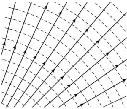
Visual representation of the action function S.
The important role of the action integral S can be illuminated by considering the case of a single point mass m moving in a time independent potential U(r). Then the action reduces to
S(q,α,t)=W(q,α)−Et
Let q1=x,q2=y,q3=z,p1=px,p2=py,p3=pz. The momentum components are given by
pi=∂W(q,α)∂qi
which corresponds to
p=∇W=∇S
That is, the time-independent Hamilton-Jacobi equation is
12m|∇W|2+U(r)=E
This implies that the particle momentum is given by the gradient of Hamilton’s characteristic function and is perpendicular to surfaces of constant W as illustrated in Figure 15.4.1. The constant W surfaces are time dependent as given by Equation ???. Thus, if at time t=0 the equi-action surface S0(q,t)=W0(q,Pi)=0, then at t=1 the same surface S0(q,t)=0 now coincides with the S0(q,t)=E surface etc. That is, the equi-action surfaces move through space separately from the motion of the single point mass.
The above pictorial representation is analogous to the situation for motion of a wavefront for electromagnetic waves in optics, or matter waves in quantum physics where the wave equation separates into the form ϕ=ϕ0eiSℏ=ϕ0ei(k⋅r−ωt). Hamilton’s goal was to create a unified theory for optics that was equally applicable to particle motion in classical mechanics. Thus the optical-mechanical analogy of the Hamilton-Jacobi theory has culminated in a universal theory that describes wave-particle duality; this was a Holy Grail of classical mechanics since Newton’s time. It played an important role in development of the Schrödinger representation of quantum mechanics.
Advantages of Hamilton-Jacobi theory
Initially, only a few scientists, like Jacobi, recognized the advantages of Hamiltonian mechanics. In 1843 Jacobi made some brilliant mathematical developments in Hamilton-Jacobi theory that greatly enhanced exploitation of Hamiltonian mechanics. Hamilton-Jacobi theory now serves as a foundation for contemporary physics, such as quantum and statistical mechanics. A major advantage of Hamilton-Jacobi theory, compared to other formulations of analytic mechanics, is that it provides a single, first-order partial differential equation for the action S, which is a function of the n generalized coordinates q and time t. The generalized momenta no longer appear explicitly in the Hamiltonian in equations ???, ???. Note that the generalized momentum do not explicitly appear in the equivalent Euler-Lagrange equations of Lagrangian mechanics, but these comprise a system of n second-order, partial differential equations for the time evolution of the generalized coordinate q. Hamilton’s equations of motion are a system of 2n first-order equations for the time evolution of the generalized coordinates and their conjugate momenta.
An important advantage of the Hamilton-Jacobi theory is that it provides a formulation of classical mechanics in which motion of a particle can be represented by a wave. In this sense, the Hamilton-Jacobi equation fulfilled a long-held goal of theoretical physics, that dates back to Johann Bernoulli, of finding an analogy between the propagation of light and the motion of a particle. This goal motivated Hamilton to develop Hamiltonian mechanics. A consequence of this wave-particle analogy is that the Hamilton-Jacobi formalism featured prominently in the derivation of the Schrödinger equation during the development of quantum-wave mechanics.