
17.7: Lorentz-invariant formulations of Hamiltonian Mechanics


- Last updated
- Jun 28, 2021
- Save as PDF

( \newcommand{\kernel}{\mathrm{null}\,}\)
Extended Canonical Formalism
A Lorentz-invariant formulation of Hamiltonian mechanics can be developed that is built upon the extended Lagrangian formalism assuming that the Hamiltonian and Lagrangian are related by a Legendre transformation. That is,
H(q,p,t)=n∑μ=1pμ∂qμ∂t−L(q,∂q∂t,t)
where the generalized momentum is defined by
pμ=∂L∂(∂qμ∂t)
Struckmeier[Str08] assumes that the definitions of the extended Lagrangian L, and the extended Hamiltonian H, are related by a Legendre transformation, and are based on variational principles, analogous to the relation that exists between the conventional Lagrangian L and Hamiltonian H. The Legendre transformation requires defining the extended generalized (canonical) momentum-energy four vector P(s)=(E(s)c,p(s)). The momentum components of the momentum-energy four vector P(s)=(E(s)c,p(s)) are given by the 1≤μ≤n components using either the conventional or the extended Lagrangians as given in Equation ???
pμ(s)=∂L∂(dqμds)=∂L∂(dqμdt)
The μ=0 component of the momentum-energy four vector is given by equation (17.6.15)
p0=1c(∂L∂(dtds))=−H(pμ,qμ,t)c=−E(s)c
where E(s) represents the instantaneous generalized energy of the conventional Hamiltonian at the point s, but not the functional form of H(q(s),p(s),t(s)). That is
E(s)≢=H(q(s),p(s),t(s))
Note that E(s) does not give the function H(q,p,t). Equations ??? and (17.6.15) give that
p0(s)=−E(s)c
The extended Hamiltonian H(q,p,t,E(s)), in an extended phase space, can be defined by the Legendre transformation and the four-vector P to be
H(q,p,t,E(s))=(P⋅q)−L(q,dqds,t,dtds)=n∑μ=0pμ(dqμds)−L(q,dqds,t,dtds)=n∑μ=1pμ(dqμds)−Edtds−L(q,dqds,t,dtds)
where the p0 term has been written explicitly as −Edtds in Equation 17.7.8. The extended Hamiltonian H((q,p,t,E(s)) can carry all the information on the dynamical system that is carried by the extended Lagrangian L(q,dqds,t,dtds), if the Hesse matrix is non-singular. That is, if
det (∂2L∂(dqμds)∂(dqνds))≠0
If the extended Lagrangian L(q,dqds,t,dtds) is not homogeneous in the n+1 velocities dqμds, then the extended set of Euler-Lagrange equations (17.6.18) is not redundant. Thus equation (17.6.12) is not an identity but it can be regarded as an implicit equation that is always satisfied by the extended set of Euler-Lagrange equations. As a result, the Legendre transformation to an extended Hamiltonian exists. That is, equation (17.6.12) is identical to the Legendre transform for H((q,p,t,E(s)) which was shown to equal zero. Therefore
H(q(s),p(s),t(s),E(s))=0
which means that the extended Hamiltonian H((q,p,t,E(s)) directly defines the restricted hypersurface on which the particle motion is confined.
The extended canonical equations of motion, derived using the extended Hamiltonian H(q(s),p(s),t(s),E(s)) with the usual Hamiltonian mechanics relations, are:
∂H∂pμ=dqμds∂H∂qμ=−dpμds∂H∂t=dEds∂H∂E=−dtds
These canonical equations give that the total derivative of H((q(s),p(s),t(s),E(s)) with respect to s, is
dHds=∂H∂pμdpμds+∂H∂qμdqμds+∂H∂tdtds+∂H∂EdEds=dqμdsdpμds−dpμdsdqμds+dEdsdtds−dtdsdEds=0
That is, in contrast to the total time derivative of H(q,p,t), the total s derivative of the extended Hamiltonian H((q(s),p(s),t(s),E(s)) always vanishes, that is, H((q(s),p(s),t(s),E(s)) is autonomous which is ideal for use with Hamilton’s equations of motion. The constraints give that H((q(s),p(s),t(s),E(s))=0, (Equation ???) and dHds=0, (Equation 17.7.17) implying that the correlation between the extended and conventional Hamiltonians is given by
H((q(s),p(s),t(s),E(s))=n∑μ=1pμ(dqμds)−Edtds−L(q,dqds,t,dtds)=n∑μ=1pμ(dqμds)−Edtds−L(q,dqds,t,)dtds=n∑μ=1pμ(dqμds)−Edtds+[H(q,p,t)−n∑μ=1pμ(dqμdt)]dtds=(H(q,p,t)−E)dtds=0
since only the term with μ=0 does not cancel in Equation 17.7.8. Equations ??? and 17.7.22 give that both the left and right-hand sides of Equation 17.7.22 are zero while Equation 17.7.17 implies that H((q(s),p(s),t(s),E(s)) is a constant of motion, that is, s is a cyclic variable for H((q(s),p(s),t(s),E(s)). Formally one can consider the extended Hamiltonian is a constant which equals zero
H(q,p,t,E(s))=E(s)=0
Equations 17.7.14, 17.7.15 imply that (E,t) form a pair of canonically conjugate variables in addition to the newly-introduced canonically-conjugate variables (E(s),s). Equation 17.7.22 shows that the motion in the 2n+2 extended phase space is constrained to the surface reflecting the fact that the observed system has one less degree of freedom than used by the extended Hamiltonian.
In summary, the Lorentz-invariant extended canonical formalism leads to Hamilton’s first-order equations of motion in terms of derivatives with respect to s, where s is related to the proper time τ for a relativistic system.
Extended Poisson Bracket representation
Struckmeier[Str08] investigated the usefulness of the extended formalism when applied to the Poisson bracket representation of Hamiltonian mechanics. The extended Poisson bracket for two differentiable functions F and G is defined as
{{F,G}}=n∑j=1(∂F∂qj∂G∂pj−∂F∂pj∂G∂qj)−∂F∂t∂G∂H+∂F∂H∂G∂t
As for the conventional Poisson bracket discussed in chapter 15, the extended Poisson also leads to the fundamental Poisson bracket relations
{{qi,qj}}=0{{pi,pj}}=0{{qi,pj}}=δij
where i,j=0,1,…,n. These are identical to the non-extended fundamental Poisson brackets.
The discussion of observables in Hamiltonian mechanics in chapter 15.2.5 can be trivially expanded to the extended Poisson bracket representation. In particular, the total s derivative of the function G is given by
dGds=∂G∂s+{{G,H}}
If G commutes with the extended Hamiltonian, that is, the Poisson bracket equals zero, and if ∂G∂s=0, then dGds=0. That is, the observable G is a constant of motion.
Substitute the fundamental variables for G gives
dpμds={{pμ,H}}=−∂H∂qμdqμds={{qμ,H}}=∂H∂pμ
where i,j=0,1,…,n. These are Hamilton’s extended canonical equations of motion expressed in terms of the system evolution parameter s. The extended Poisson bracket representation is a trivial extension of the conventional canonical equations presented in chapter 15.3.
Extended canonical transformation and Hamilton-Jacobi theory
Struckmeier[Str08] presented plausible extended versions of canonical transformation and Hamilton-Jacobi theories that can be used to provide a Lorentz-invariant formulation of Hamiltonian mechanics for relativistic one-body systems. A detailed description can be found in Struckmeier[Str08].1
Validity of the extended Hamilton-Lagrange formalism
It has been shown that the extended Lagrangian and Hamiltonian formalism, based on the parametric model of Lanczos[La49], leads to a plausible manifestly-covariant approach for the one-body system. The general features developed for handling Lagrangian and Hamiltonian mechanics carry over to the Special Theory of Relativity assuming the use of a non-standard, extended Lagrangian or Hamiltonian. This expansion of the range of validity of the well-known Hamiltonian and Lagrangian mechanics into the relativistic domain is important, and reduces any Lorentz transformation to a canonical transformation. The validity of this extended Hamilton-Lagrange formalism has been criticized, and problems exist extending this approach to the N-body system for N>1. For example, as discussed by Goldstein[Go50] and Johns[Jo05], each of the N moving bodies have their own world lines and momenta. Defining the total momentum P requires knowing simultaneously the momenta of the individual bodies, but simultaneity is body dependent and thus even the total momentum is not a simple four vector. A general method is required that will allow using a manifestly-covariant Lagrangian or Hamiltonian for the N-body system. For the one-body system, the extended Hamilton-Lagrange formalism provides a powerful and logical approach to exploit analytical mechanics in the relativistic domain that retains the form of the conventional Lagrangian/Hamiltonian formalisms. Note that Noether’s theorem relating energy and time is readily apparent using the extended formalism.
Example 17.7.1: The Bohr-Sommerfeld hydrogen atom
The classical relativistic hydrogen atom was first solved by Sommerfeld in 1916. Sommerfeld used Bohr’s “old quantum theory” plus Hamiltonian mechanics to make an important step in the development of quantum mechanics by obtaining the first-order expressions for the fine structure of the hydrogen atom. As in the non-relativistic case, the motion is confined to a plane allowing use of planar polar coordinates. Thus the relativistic Lagrangian is given by
L=−mc2γ−U=−mc2√1−˙r2+r2˙θ2c2+ke2r
The canonical momenta are given by
pθ=∂L∂˙θ=mγr2˙θpr=∂L∂˙r=mγ˙r˙pθ=∂L∂θ=0˙pr=∂L∂r=mγr˙θ2+ke2r2
As for the non-relativistic case, θ is a cyclic variable and thus the angular momentum pθ=mγr2˙θ is conserved.
The relativistic Hamiltonian for the Coulomb potential between an electron and the proton, assuming that the motion is confined to a plane, which allows use of planar polar coordinates, leads to
H=√p2rc2+p2θc2r2+m2c4−ke2r
The same equations of motion are obtained using Hamiltonian mechanics, that is:
˙θ=∂H∂pθ=pθmγr2˙r=∂H∂pr=prmγ˙pθ=−∂H∂θ=0˙pr=−∂H∂r=mγr˙θ2+ke2r2
The radial dependence can be solved using either Lagrangian or Hamiltonian mechanics, but the solution is non-trivial. Using the same techniques applied to solve Kepler’s problem, leads to the radial solution
r=q1+ϵcos[Γ(θ−θ0]Γ=√1−e4c2p2θq=c2Γ2p2θe2Eϵ=√1+Γ2(1−m2c4E2)1−Γ2
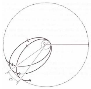
The apses are rmin=q(1+ϵ) for Γ(θ−θ0)=0, 2π,4π, and rmax=q(1−ϵ) for Γ(θ−θ0)=π,3π,. The perihelion advances between cycles due to the change in relativistic mass during the trajectory as shown in (Figure 17.7.1). This precession leads to the fine structure observed in the optical spectra of the hydrogen atom. The same precession of the perihelion occurs for planetary motion, however, there is a comparable size effect due to gravity that requires use of general relativity to compute the trajectories.
1Note that Greiner[Gr10] includes a reproduction of the Struckmeier paper[Str08].