
19.5: Appendix - Coordinate transformations
- Page ID
- 9688

\( \newcommand{\vecs}[1]{\overset { \scriptstyle \rightharpoonup} {\mathbf{#1}} } \)
\( \newcommand{\vecd}[1]{\overset{-\!-\!\rightharpoonup}{\vphantom{a}\smash {#1}}} \)
\( \newcommand{\dsum}{\displaystyle\sum\limits} \)
\( \newcommand{\dint}{\displaystyle\int\limits} \)
\( \newcommand{\dlim}{\displaystyle\lim\limits} \)
\( \newcommand{\id}{\mathrm{id}}\) \( \newcommand{\Span}{\mathrm{span}}\)
( \newcommand{\kernel}{\mathrm{null}\,}\) \( \newcommand{\range}{\mathrm{range}\,}\)
\( \newcommand{\RealPart}{\mathrm{Re}}\) \( \newcommand{\ImaginaryPart}{\mathrm{Im}}\)
\( \newcommand{\Argument}{\mathrm{Arg}}\) \( \newcommand{\norm}[1]{\| #1 \|}\)
\( \newcommand{\inner}[2]{\langle #1, #2 \rangle}\)
\( \newcommand{\Span}{\mathrm{span}}\)
\( \newcommand{\id}{\mathrm{id}}\)
\( \newcommand{\Span}{\mathrm{span}}\)
\( \newcommand{\kernel}{\mathrm{null}\,}\)
\( \newcommand{\range}{\mathrm{range}\,}\)
\( \newcommand{\RealPart}{\mathrm{Re}}\)
\( \newcommand{\ImaginaryPart}{\mathrm{Im}}\)
\( \newcommand{\Argument}{\mathrm{Arg}}\)
\( \newcommand{\norm}[1]{\| #1 \|}\)
\( \newcommand{\inner}[2]{\langle #1, #2 \rangle}\)
\( \newcommand{\Span}{\mathrm{span}}\) \( \newcommand{\AA}{\unicode[.8,0]{x212B}}\)
\( \newcommand{\vectorA}[1]{\vec{#1}} % arrow\)
\( \newcommand{\vectorAt}[1]{\vec{\text{#1}}} % arrow\)
\( \newcommand{\vectorB}[1]{\overset { \scriptstyle \rightharpoonup} {\mathbf{#1}} } \)
\( \newcommand{\vectorC}[1]{\textbf{#1}} \)
\( \newcommand{\vectorD}[1]{\overrightarrow{#1}} \)
\( \newcommand{\vectorDt}[1]{\overrightarrow{\text{#1}}} \)
\( \newcommand{\vectE}[1]{\overset{-\!-\!\rightharpoonup}{\vphantom{a}\smash{\mathbf {#1}}}} \)
\( \newcommand{\vecs}[1]{\overset { \scriptstyle \rightharpoonup} {\mathbf{#1}} } \)
\(\newcommand{\longvect}{\overrightarrow}\)
\( \newcommand{\vecd}[1]{\overset{-\!-\!\rightharpoonup}{\vphantom{a}\smash {#1}}} \)
\(\newcommand{\avec}{\mathbf a}\) \(\newcommand{\bvec}{\mathbf b}\) \(\newcommand{\cvec}{\mathbf c}\) \(\newcommand{\dvec}{\mathbf d}\) \(\newcommand{\dtil}{\widetilde{\mathbf d}}\) \(\newcommand{\evec}{\mathbf e}\) \(\newcommand{\fvec}{\mathbf f}\) \(\newcommand{\nvec}{\mathbf n}\) \(\newcommand{\pvec}{\mathbf p}\) \(\newcommand{\qvec}{\mathbf q}\) \(\newcommand{\svec}{\mathbf s}\) \(\newcommand{\tvec}{\mathbf t}\) \(\newcommand{\uvec}{\mathbf u}\) \(\newcommand{\vvec}{\mathbf v}\) \(\newcommand{\wvec}{\mathbf w}\) \(\newcommand{\xvec}{\mathbf x}\) \(\newcommand{\yvec}{\mathbf y}\) \(\newcommand{\zvec}{\mathbf z}\) \(\newcommand{\rvec}{\mathbf r}\) \(\newcommand{\mvec}{\mathbf m}\) \(\newcommand{\zerovec}{\mathbf 0}\) \(\newcommand{\onevec}{\mathbf 1}\) \(\newcommand{\real}{\mathbb R}\) \(\newcommand{\twovec}[2]{\left[\begin{array}{r}#1 \\ #2 \end{array}\right]}\) \(\newcommand{\ctwovec}[2]{\left[\begin{array}{c}#1 \\ #2 \end{array}\right]}\) \(\newcommand{\threevec}[3]{\left[\begin{array}{r}#1 \\ #2 \\ #3 \end{array}\right]}\) \(\newcommand{\cthreevec}[3]{\left[\begin{array}{c}#1 \\ #2 \\ #3 \end{array}\right]}\) \(\newcommand{\fourvec}[4]{\left[\begin{array}{r}#1 \\ #2 \\ #3 \\ #4 \end{array}\right]}\) \(\newcommand{\cfourvec}[4]{\left[\begin{array}{c}#1 \\ #2 \\ #3 \\ #4 \end{array}\right]}\) \(\newcommand{\fivevec}[5]{\left[\begin{array}{r}#1 \\ #2 \\ #3 \\ #4 \\ #5 \\ \end{array}\right]}\) \(\newcommand{\cfivevec}[5]{\left[\begin{array}{c}#1 \\ #2 \\ #3 \\ #4 \\ #5 \\ \end{array}\right]}\) \(\newcommand{\mattwo}[4]{\left[\begin{array}{rr}#1 \amp #2 \\ #3 \amp #4 \\ \end{array}\right]}\) \(\newcommand{\laspan}[1]{\text{Span}\{#1\}}\) \(\newcommand{\bcal}{\cal B}\) \(\newcommand{\ccal}{\cal C}\) \(\newcommand{\scal}{\cal S}\) \(\newcommand{\wcal}{\cal W}\) \(\newcommand{\ecal}{\cal E}\) \(\newcommand{\coords}[2]{\left\{#1\right\}_{#2}}\) \(\newcommand{\gray}[1]{\color{gray}{#1}}\) \(\newcommand{\lgray}[1]{\color{lightgray}{#1}}\) \(\newcommand{\rank}{\operatorname{rank}}\) \(\newcommand{\row}{\text{Row}}\) \(\newcommand{\col}{\text{Col}}\) \(\renewcommand{\row}{\text{Row}}\) \(\newcommand{\nul}{\text{Nul}}\) \(\newcommand{\var}{\text{Var}}\) \(\newcommand{\corr}{\text{corr}}\) \(\newcommand{\len}[1]{\left|#1\right|}\) \(\newcommand{\bbar}{\overline{\bvec}}\) \(\newcommand{\bhat}{\widehat{\bvec}}\) \(\newcommand{\bperp}{\bvec^\perp}\) \(\newcommand{\xhat}{\widehat{\xvec}}\) \(\newcommand{\vhat}{\widehat{\vvec}}\) \(\newcommand{\uhat}{\widehat{\uvec}}\) \(\newcommand{\what}{\widehat{\wvec}}\) \(\newcommand{\Sighat}{\widehat{\Sigma}}\) \(\newcommand{\lt}{<}\) \(\newcommand{\gt}{>}\) \(\newcommand{\amp}{&}\) \(\definecolor{fillinmathshade}{gray}{0.9}\)Coordinate systems can be translated, or rotated with respect to each other as well as being subject to spatial inversion or time reversal. Scalars, vectors, and tensors are defined by their transformation properties under rotation, spatial inversion and time reversal, and thus such transformations play a pivotal role in physics.
Translational transformations
Translational transformations are involved frequently for transforming between the center of mass and laboratory frames for reaction kinematics as well as when performing vector addition of central forces for the cases where the centers are displaced. Both the classical Galilean transformation or the relativistic Lorentz transformation are handled the same way. Consider two parallel orthonormal coordinate frames where the origin of \(F^{\prime} (x^{\prime}, y^{\prime}, z^{\prime} )\) is displaced by a time dependent vector \(\mathbf{a}(t)\) from the origin of frame \(F (x, y, z)\). Then the Galilean transformation for a vector \(\mathbf{r}\) in frame \(\mathbf{F}\) to \(\mathbf{r}^{\prime}\) in frame \(F^{\prime}\) is given by
\[\mathbf{r} (x^{\prime}, y^{\prime}, z^{\prime} ) = \mathbf{r} (x, y, z) +\mathbf{a}(t) \label{D.1}\]
The velocities for a moving frame are given by the vector difference of the velocity in a stationary frame, and the velocity of the origin of the moving frame. Linear accelerations can be handled similarly.
Rotational transformations
Rotation matrix
Rotational transformations of the coordinate system are used extensively in physics. The transformation properties of fields under rotation define the scalar and vector properties of fields, as well as rotational symmetry and conservation of angular momentum.
Rotation of the coordinate frame does not change the value of any scalar observable such as mass, temperature etc. That is, transformation of a scalar quantity is invariant under coordinate rotation from \(x, y, z \rightarrow x^{\prime}, y^{\prime}, z^{\prime}\).
\[\phi (x^{\prime} y^{\prime} z^{\prime} ) = \phi (xyz) \label{D.2}\]
By contrast, the components of a vector along the coordinate axes change under rotation of the coordinate axes. This difference in transformation properties under rotation between a scalar and a vector is important and defines both scalars and a vectors.
Matrix mechanics, described in appendix \(19.1\), provides the most convenient way to handle coordinate rotations. The transformation matrix, between coordinate systems having differing orientations is called the rotation matrix. This transforms the components of any vector with respect to one coordinate frame to the components with respect to a second coordinate frame rotated with respect to the first frame.
Assume a point \(P\) has coordinates \((x_1, x_2, x_3)\) with respect to a certain coordinate system. Consider rotation to another coordinate frame for which the point \(P\) has coordinates \((x^{\prime}_1, x^{\prime}_2, x^{\prime}_3)\) and assume that the origins of both frames coincide. Rotation of a frame does not change the vector, only the vector components of the unit basis states. Therefore
\[\mathbf{x} = \mathbf{\hat{e}}^{\prime}_1 x^{\prime}_1 + \mathbf{\hat{e}}^{\prime}_2 x^{\prime}_2 + \mathbf{\hat{e}}^{\prime}_3x^{\prime}_3 = \mathbf{\hat{e}}_1x_1 + \mathbf{\hat{e}}_2x_2 + \mathbf{\hat{e}}_3x_3 \label{D.3}\]
Note that if one designates that the unit vectors for the unprimed coordinate frame are \((\mathbf{\hat{e}}_1, \mathbf{\hat{e}}_2, \mathbf{\hat{e}}_3)\) and for the primed coordinate frame \((\mathbf{\hat{e}}^{\prime}_1, \mathbf{\hat{e}}^{\prime}_2, \mathbf{\hat{e}}^{\prime}_3)\), then taking the scalar product of Equation \ref{D.3} sequentially with each of the unit base vectors \((\mathbf{\hat{e}}^{\prime}_1, \mathbf{\hat{e}}^{\prime}_2, \mathbf{\hat{e}}^{\prime}_3)\) leads to the following three relations
\[x^{\prime}_1 = (\mathbf{\hat{e}}^{\prime}_1 \cdot \mathbf{\hat{e}}_1)x_1 + (\mathbf{\hat{e}}^{\prime}_1 \cdot \mathbf{\hat{e}}_2)x_2 + (\mathbf{\hat{e}}^{\prime}_1 \cdot \mathbf{\hat{e}}_3)x_3 \label{D.4} \\ x^{\prime}_2 = (\mathbf{\hat{e}}^{\prime}_2 \cdot \mathbf{\hat{e}}_1)x_1 + (\mathbf{\hat{e}}^{\prime}_2 \cdot \mathbf{\hat{e}}_2)x_2 + (\mathbf{\hat{e}}^{\prime}_2 \cdot \mathbf{\hat{e}}_3)x_3 \\ x^{\prime}_3 = (\mathbf{\hat{e}}^{\prime}_3 \cdot \mathbf{\hat{e}}_1)x_1 + (\mathbf{\hat{e}}^{\prime}_3 \cdot \mathbf{\hat{e}}_2)x_2 + (\mathbf{\hat{e}}^{\prime}_3 \cdot \mathbf{\hat{e}}_3)x_3 \]
Note that the \( (\mathbf{\hat{e}}^{\prime}_i \cdot \mathbf{\hat{e}}_j )\) are the direction cosines as defined by the scalar product of two unit vectors for axes \(i, j\), that is, they are the cosine of the angle between the two unit vectors.
Equation \ref{D.4} can be written in matrix form as
\[\mathbf{x}^{\prime} = \boldsymbol{\lambda} \cdot \mathbf{x} \label{D.5}\]
where the “\( \cdot \)” means the inner matrix product of the rotation matrix \(\boldsymbol{\lambda}\) and the vector \(\mathbf{x}\) where
\[\mathbf{x}^{\prime} \equiv \begin{pmatrix} x^{\prime}_1 \\ x^{\prime}_2 \\ x^{\prime}_3 \end{pmatrix} \quad \mathbf{x} \equiv \begin{pmatrix} x_1 \\ x_2 \\ x_3 \end{pmatrix} \quad \boldsymbol{\lambda} \equiv \begin{pmatrix} \mathbf{\hat{e}}^{\prime}_1 \cdot \mathbf{\hat{e}}_1 & \mathbf{\hat{e}}^{\prime}_1 \cdot \mathbf{\hat{e}}_2 & \mathbf{\hat{e}}^{\prime}_1 \cdot \mathbf{\hat{e}}_3 \\ \mathbf{\hat{e}}^{\prime}_2 \cdot \mathbf{\hat{e}}_1 & \mathbf{\hat{e}}^{\prime}_2 \cdot \mathbf{\hat{e}}_2 & \mathbf{\hat{e}}^{\prime}_2 \cdot \mathbf{\hat{e}}_3 \\ \mathbf{\hat{e}}^{\prime}_3 \cdot \mathbf{\hat{e}}_1 & \mathbf{\hat{e}}^{\prime}_3 \cdot \mathbf{\hat{e}}_2 & \mathbf{\hat{e}}^{\prime}_3 \cdot \mathbf{\hat{e}}_3 \end{pmatrix} \label{D.6}\]
The inverse procedure is obtained by multiplying Equation \ref{D.3} successively by one of the unit basis vectors \((\mathbf{\hat{e}}_1, \mathbf{\hat{e}}_2, \mathbf{\hat{e}}_3)\) leading to three equations
\[x_1 = (\mathbf{\hat{e}}_1 \cdot \mathbf{\hat{e}}^{\prime}_1) x^{\prime}_1 + (\mathbf{\hat{e}}_1 \cdot \mathbf{\hat{e}}^{\prime}_2) x^{\prime}_2 + (\mathbf{\hat{e}}_1 \cdot \mathbf{\hat{e}}^{\prime}_3) x^{\prime}_3 \label{D.7} \\ x_2 = (\mathbf{\hat{e}}_2 \cdot \mathbf{\hat{e}}^{\prime}_1)x^{\prime}_1 + (\mathbf{\hat{e}}_2 \cdot \mathbf{\hat{e}}^{\prime}_2)x^{\prime}_2 + (\mathbf{\hat{e}}_2 \cdot \mathbf{\hat{e}}^{\prime}_3)x^{\prime}_3 \\ x_3 = (\mathbf{\hat{e}}_3 \cdot \mathbf{\hat{e}}^{\prime}_1)x^{\prime}_1 + (\mathbf{\hat{e}}_3 \cdot \mathbf{\hat{e}}^{\prime}_2)x^{\prime}_2 + (\mathbf{\hat{e}}_3 \cdot \mathbf{\hat{e}}^{\prime}_3)x^{\prime}_3 \]
Equation \ref{D.7} can be written in matrix form as
\[\mathbf{x} = \boldsymbol{\lambda}^T \cdot \mathbf{x}^{\prime} \label{D.8}\]
where \(\boldsymbol{\lambda}^T\) is the transpose of \(\boldsymbol{\lambda}\).
Note that substituting Equation \ref{D.5} into Equation \ref{D.8} gives
\[\mathbf{x} = \boldsymbol{\lambda}^T \cdot (\boldsymbol{\lambda} \cdot \mathbf{x}) = \left( \boldsymbol{\lambda}^T \cdot \boldsymbol{\lambda} \right) \cdot \mathbf{x} \label{D.9}\]
Thus
\[\left( \boldsymbol{\lambda}^T \cdot \boldsymbol{\lambda} \right) = \mathbb{I} \nonumber\]
where \(\mathbb{I}\) is the identity matrix. This implies that the rotation matrix \(\boldsymbol{\lambda}\) is orthogonal with \(\boldsymbol{\lambda}^T = \boldsymbol{\lambda}^{−1}\).
It is convenient to rename the elements of the rotation matrix to be
\[\lambda_{ij} \equiv (\mathbf{\hat{e}}^{\prime}_i \cdot \mathbf{\hat{e}}_j ) \label{D.10}\]
so that the rotation matrix is written more compactly as
\[\boldsymbol{\lambda} \equiv \begin{pmatrix}\lambda_{11} & \lambda_{12} & \lambda_{13} \\ \lambda_{21} & \lambda_{22} & \lambda_{23} \\ \lambda_{31} & \lambda_{32} & \lambda_{33} \end{pmatrix} \nonumber\]
and Equation \ref{D.4} becomes
\[x^{\prime}_1 = \lambda_{11}x_1 + \lambda_{12}x_2 + \lambda_{13}x_3 \label{D.11} \\ x^{\prime}_2 = \lambda_{21}x_1 + \lambda_{22}x_2 + \lambda_{23}x_3 \\ x^{\prime}_3 = \lambda_{31}x_1 + \lambda_{32}x_2 + \lambda_{33}x_3 \]
Consider an arbitrary rotation through an angle \(\theta \). Equations \ref{D.10} and \ref{D.11} can be used to relate six of the nine quantities \(\lambda_{ij}\) in the rotation matrix, so only three of the quantities are independent. That is, because of Equation \ref{D.11} we have three equations which ensure that the transformation is unitary.
\[\lambda^2_{i1} + \lambda^2_{i2} + \lambda^2_{i3} = 1 \label{D.12}\]
Also requiring that the axes be orthogonal gives three equations
\[\sum_j \lambda_{ij} \lambda_{kj} = 0, \quad i \neq k \label{D.13}\]
These six relations can be expressed as
\[\sum_j \lambda_{ij} \lambda_{kj} = \delta_{ik} \label{D.14}\]
The fact that the rotation matrix should have three independent quantities is due to the fact that all rotations can be expressed in terms of rotations about three orthogonal axes.
Example \(\PageIndex{1}\)
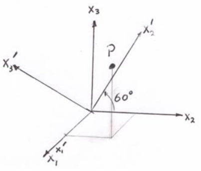
Consider a point \(P(x_1, x_2, x_3) = P(3, 4, 5)\) in the unprimed coordinate system. Consider the same point \(P(x^{\prime}_1, x^{\prime}_2, x^{\prime}_3)\) in the primed coordinate system which has been rotated by an angle \(60^{\circ}\) about the \(x_1\) axis as shown. The direction cosines \(\lambda_{i^{\prime}j} = \cos ( \theta_{i^{\prime}j} )\) can be determined from the figure to be the following
| \(i^{\prime}\) | \(j\) | \(\theta_{i^{\prime}j}\) | \(\lambda_{i^{\prime}j} = \cos (\theta_{i^{\prime}j})\) |
|---|---|---|---|
| 1 | 1 | 0 | 1 |
| 1 | 2 | 90 | 0 |
| 1 | 3 | 90 | 0 |
| 2 | 1 | 90 | 0 |
| 2 | 2 | 60 | 0.500 |
| 2 | 3 | 90-60 | 0.866 |
| 3 | 1 | 90 | 0 |
| 3 | 2 | 90+60 | -0.866 |
| 3 | 3 | 60 | 0.500 |
Thus the rotation matrix is
\[\lambda =\begin{pmatrix} 1. & 0 & 0 \\ 0 & 0.500 & 0.866 \\ 0 & −0.866 & 0.500 \end{pmatrix} \nonumber\]
The transform point \(P^{\prime} (x^{\prime}_1, x^{\prime}_2, x^{\prime}_3)\) therefore is given by
\[\begin{pmatrix}x^{\prime}_1 \\ x^{\prime}_2 \\ x^{\prime}_3 \end{pmatrix} =\begin{pmatrix}1. & 0 & 0 \\ 0 & 0.500 & 0.866 \\ 0 & −0.866 & 0.500 \end{pmatrix} \cdot \begin{pmatrix} 3 \\ 4 \\ 5 \end{pmatrix} =\begin{pmatrix} 3 \\ 6.330 \\ −0.964 \end{pmatrix} \nonumber\]
Note that the radial coordinate \(r_P= r^{\prime}_P= \sqrt{50}\). That is, the rotational transformation is unitary and thus the magnitude of the vector is unchanged.
Example \(\PageIndex{2}\): Proof that a rotation matrix is orthogonal
Consider the rotation matrix
\[\boldsymbol{\lambda} = \frac{1}{9} \begin{pmatrix} 4 & 7 & −4 \\ 1 & 4 & 8 \\ 8 & −4 & 1 \end{pmatrix} \nonumber\]
The product
\[\boldsymbol{\lambda}^T \cdot \boldsymbol{\lambda} = \frac{1}{ 81} \begin{pmatrix} 4 & 1 & 8 \\ 7 & 4 & −4 \\ −4 & 8 & 1 \end{pmatrix} \cdot \begin{pmatrix} 4 & 7 & −4 \\ 1 & 4 & 8 \\ 8 & −4 & 1 \end{pmatrix} = \frac{1}{ 81} \begin{pmatrix} 81 & 0 & 0 \\ 0 & 81 & 0 \\ 0 & 0 & 81 \end{pmatrix} = 1 \nonumber\]
which implies that \(\lambda\) is orthogonal.
Finite rotations
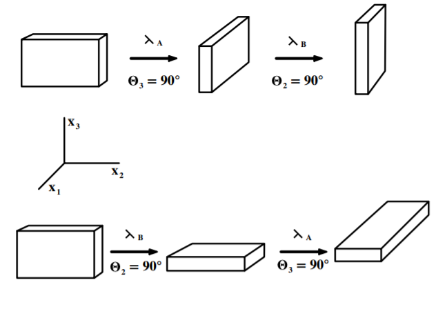
Consider two finite \(90^{\circ}\) rotations \(\lambda_{A}\) and \(\lambda_{B}\) illustrated in Figure \(\PageIndex{2}\). The \(\lambda_{A}\) rotation is \(90^{\circ}\) around the \(x_3\) axis in a right-handed direction as shown. In such a rotation the axes transform to \(x^{\prime}_1 = x_2, x^{\prime}_2 = −x_1, x^{\prime}_3 = x_3\) and the rotation matrix is
\[\boldsymbol{\lambda}_A =\begin{pmatrix} 0 & 1 & 0 \\ −1 & 0 & 0 \\ 0 & 0 & 1 \end{pmatrix} \label{D.15}\]
The second rotation \(\boldsymbol{\lambda}_B\) is a right-handed rotation about the \(x^{\prime}_1\) axis which formerly was the \(x_2\) axis. Then \(x^{"}_1 = x^{\prime}_2, x^{"}_2 = −x^{\prime}_1, x^{"}_3 = x^{\prime}_3\) and the rotation matrix is
\[\boldsymbol{\lambda}_B =\begin{pmatrix} 1 & 0 & 0 \\ 0 & 0 & 1 \\ 0 & −1 & 0 \end{pmatrix} \label{D.16}\]
Consider the product of these two finite rotations which corresponds to a single rotation matrix \(\boldsymbol{\lambda}_{AB}\)
\[ \boldsymbol{\lambda}_{AB} = \boldsymbol{\lambda}_B \boldsymbol{\lambda}_A \label{D.17}\]
That is:
\[\boldsymbol{\lambda}_{AB} =\begin{pmatrix} 1 & 0 & 0 \\ 0 & 0 & 1 \\ 0 & −1 & 0 \end{pmatrix} \begin{pmatrix} 0 & 1 & 0 \\ −1 & 0 & 0 \\ 0 & 0 & 1 \end{pmatrix} = \begin{pmatrix} 0 & 1 & 0 \\ 0 & 0 & 1 \\ 1 & 0 & 0 \end{pmatrix} \label{D.18}\]
Now consider that the order of these two rotations is reversed.
\[\boldsymbol{\lambda}_{BA} = \boldsymbol{\lambda}_A \boldsymbol{\lambda}_B \label{D.19}\]
That is:
\[\boldsymbol{\lambda}_{BA} = \begin{pmatrix} 0 & 1 & 0 \\ −1 & 0 & 0 \\ 0 & 0 & 1 \end{pmatrix} \begin{pmatrix} 1 & 0 & 0 \\ 0 & 0 & 1 \\ 0 & −1 & 0 \end{pmatrix} = \begin{pmatrix} 0 & 0 & 1 \\ −1 & 0 & 0 \\ 0 & −1 & 0 \end{pmatrix} \neq \boldsymbol{\lambda}_{AB} \label{D.20}\]
An entirely different orientation results as illustrated in Figure \(\PageIndex{2}\).
This behavior of finite rotations is a consequence of the fact that finite rotations do not commute, that is, reversing the order does not give the same answer. Thus, if we associate the vectors \(\mathbf{A}\) and \(\mathbf{B}\) with these rotations, then it implies that the vector product \(\mathbf{AB} \neq \mathbf{BA}\). That is, for finite rotation matrices, the product does not behave like for true vectors since they do not commute.
Infinitessimal rotations
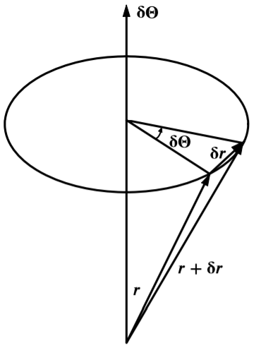
Infinitessimal rotations do not suffer from the noncommutation defect of finite rotations. If the position vector of a point changes from \(\mathbf{r}\) to \(\mathbf{r} + \delta \mathbf{r}\) then the geometrical situation is represented correctly by
\[\delta \mathbf{r} = \delta \boldsymbol{\theta} \times \mathbf{r} \label{D.21}\]
where \(\delta \boldsymbol{\theta}\) is a quantity whose magnitude is equal to the infinitessimal rotation angle and which has a direction along the instantaneous axis of rotation as illustrated in Figure \(\PageIndex{3}\).
The infinitessimal angle \(\delta \boldsymbol{\theta}\) is a vector which is shown by proving that two infinitessimal rotations \(\delta \boldsymbol{\theta}_1\) and \(\delta \boldsymbol{\theta}_2\) commute. The change in position vectors of the point are
\[\delta \mathbf{r}_1 = \delta \boldsymbol{\theta}_1 \times \mathbf{r} \label{D.22}\]
and
\[\delta \mathbf{r}_2 = \delta \boldsymbol{\theta}_2 \times (\mathbf{r} + \delta \mathbf{r}_1) \label{D.23}\]
Thus the final position vector for \(\delta \boldsymbol{\theta}_1\) followed by \(\delta \boldsymbol{\theta}_2\) is
\[\mathbf{r} + \delta \mathbf{r}_1 + \delta \mathbf{r}_2 = \mathbf{r} + \delta \boldsymbol{\theta}_1 \times \mathbf{r} + \delta \boldsymbol{\theta}_2 \times ( \mathbf{r} + \delta \mathbf{r}_1) \label{D.24}\]
Assuming that the second-order infinitessimals can be ignored gives
\[\mathbf{r} + \delta \mathbf{r}_1 + \delta \mathbf{r}_2 = \mathbf{r} + \delta \boldsymbol{\theta}_1 \times \mathbf{}\mathbf{r} + \delta \boldsymbol{\theta}_2 \times \mathbf{r} \label{D.25}\]
Consider now the inverse order of rotations.
\[\mathbf{r} + \delta \mathbf{r}_2 + \delta \mathbf{r}_1 = \mathbf{r} + \delta \boldsymbol{\theta}_2 \times \mathbf{r} + \delta \boldsymbol{\theta}_1 \times (\mathbf{r} + \delta \mathbf{r}_2) \label{D.26}\]
Again, neglecting the second-order infinitessimals gives
\[\mathbf{r} + \delta \mathbf{r}_2 + \delta \mathbf{r}_1 = \mathbf{r} + \delta \boldsymbol{\theta}_2 \times \mathbf{r} + \delta \boldsymbol{\theta}_1 \times \mathbf{r} \label{D.27}\]
Note that the products of these two infinitessimal rotations, \ref{D.25} and \ref{D.27} are identical. That is, assuming that second-order infinitessimals can be neglected, then the infinitessimal rotations commute, and thus \(\delta \boldsymbol{\theta}_1\) and \(\delta \boldsymbol{\theta}_2\) are correctly represented by vectors.
The fact that \(\delta \boldsymbol{\theta}\) is a vector allows angular velocity to be represented by a vector. That is, angular velocity is the ratio of an infinitessimal rotation to an infinitessimal time.
\[\boldsymbol{\omega} = \frac{\delta \boldsymbol{\theta}}{ \delta t } \label{D.28}\]
Note that this implies that the velocity of the point can be expressed as
\[\mathbf{v} = \frac{\delta \mathbf{r}}{ \delta t} = \frac{\delta \boldsymbol{\theta}}{ \delta t} \times \mathbf{r} = \boldsymbol{\omega} \times \mathbf{r} \label{D.29}\]
Proper and improper rotations
The requirement that the coordinate axes be orthogonal, and that the transformation be unitary, leads to the relation between the components of the rotation matrix.
\[\sum_j \lambda_{ij} \lambda_{kj} = \delta_{ik} \label{D.30}\]
It was shown in equation \((19.1.12)\) that, for such an orthogonal matrix, the inverse matrix \(\lambda^{−1}\) equals the transposed matrix \(\lambda^T\)
\[\boldsymbol{\lambda}^{−1} = \boldsymbol{\lambda}^T \nonumber\]
Inserting the orthogonality relation for the rotation matrix leads to the fact that the square of the determinant of the rotation matrix equals one,
\[|\lambda |^2 = 1 \label{D.31}\]
that is
\[|\lambda | = \pm 1 \label{D.32}\]
A proper rotation is the rotation of a normal vector and has
\[|\lambda | = +1 \label{D.33}\]
An improper rotation corresponds to
\[|\lambda | = −1 \label{D.34}\]
An improper rotation implies a rotation plus a spatial reflection which cannot be achieved by any combination of only rotations.
Consider the cross product of two vectors \( \mathbf{c} = \mathbf{a} \times \mathbf{b}\). It can be shown that the cross product behaves under rotation as:
\[c^{\prime}_i = |\lambda | \sum_j \lambda_{ij} c_j \label{D.35}\]
For all proper rotations the determinant of \(\lambda = +1\) and thus the cross product also acts like a proper vector under rotation. This is not true for improper rotations where \(|\lambda | = −1\).
Spatial inversion transformation
Spatial inversion, that is, mirror reflection, corresponds to reflection of all coordinate vectors, \(\widehat{\mathbf{i}} = − \widehat{\mathbf{i}}\), \(\widehat{\mathbf{j}} = − \widehat{\mathbf{j}}\), and \(\widehat{\mathbf{k}} = − \widehat{\mathbf{k}}\). Such a transformation corresponds to the transformation matrix
\[\boldsymbol{\lambda} =\begin{pmatrix} −1 & 0 & 0 \\ 0 & −1 & 0 \\ 0 & 0 & −1 \end{pmatrix} = −\begin{pmatrix} 1 & 0 & 0 \\ 0 & 1 & 0 \\ 0 & 0 & 1 \end{pmatrix} \label{D.36}\]
Thus \(|\lambda | = −1\), that is, it corresponds to an improper rotation. A spatial inversion for two vectors \(\mathbf{A}(r)\) and \(\mathbf{B}(r)\) correspond to
\[\mathbf{A}(r) = −\mathbf{A}(-r) \label{D.37} \\ \mathbf{B}(r) = −\mathbf{B}(-r) \]
That is, normal polar vectors change sign under spatial reflection. However, the cross product \(\mathbf{C} = \mathbf{A} \times \mathbf{B}\) does not change sign under spatial inversion since the product of the two minus signs is positive. That is,
\[\mathbf{C}(r)=+\mathbf{C}(-r) \label{D.38}\]
Thus the cross product behaves differently from a polar vector. This improper behavior is characteristic of an axial vector, which also is called a pseudovector.
Examples of pseudovectors are angular momentum, spin, magnetic field etc. These pseudovectors are defined using the right-hand rule and thus have handedness. For a right-handed system
\[\mathbf{C}_R = \mathbf{A} \times \mathbf{B} \label{D.39}\]
Changing to a left-handed system leads to
\[\mathbf{C}_L = \mathbf{B} \times \mathbf{A} = −\mathbf{A} \times \mathbf{B} \label{D.40}\]
That is, handedness corresponds to a definite ordering of the cross product. Proper orthogonal transformations are said to preserve chirality (Greek for handedness) of a coordinate system.
An example of the use of the right-handed system is the usual definition of cartesian unit vectors,
\[\widehat{\mathbf{i}} \times \widehat{\mathbf{j}} = \widehat{\mathbf{k}} \label{D.41}\]
An obvious question to be asked, is the handedness of a coordinate system merely a mathematical curiosity or does it have some deep underlying significance? Consider the Lorentz force
\[\mathbf{F} = q (\mathbf{E} + \mathbf{v} \times \mathbf{B}) \label{D.42}\]
Since force and velocity are proper vectors then the magnetic \(\mathbf{B}\) field must be a pseudo vector. Note that calculation of the \(\mathbf{B}\) field occurs only in cross products such as,
\[\boldsymbol{\nabla} \times \mathbf{B} = \mu \mathbf{j} \label{D.43}\]
where the current density \(\mathbf{j}\) is a proper vector. Another example is the Biot-Savart Law which expresses \(\mathbf{B}\) as
\[d\mathbf{B} = \frac{\mu_oI}{4\pi} \frac{ d\mathbf{l} \times \mathbf{r}}{r^2} \label{D.44}\]
Thus even though \(\mathbf{B}\) is a pseudo vector, the force \(\mathbf{F}\) remains a proper vector. Thus if a left-handed coordinate definition of \(\mathbf{B}_L = \frac{\mu_oI}{4\pi} \frac{ \mathbf{r} \times d\mathbf{l}}{r^2}\) is used in \ref{D.44}, and \(\mathbf{F} = q (\mathbf{E} + \mathbf{B}_L \times \mathbf{v})\) in \ref{D.42}, then the same final physical result would be obtained.
It was long thought that the laws of physics were symmetric with respect to spatial inversion ( i.e. mirror reflection), meaning that the choice between a left-handed and right-handed representations (chirality) was arbitrary. This is true for gravitational, electromagnetic and the strong force, and is called the conservation of parity. The fourth fundamental force in nature, the weak force, violates parity and favours handedness. It turns out that right-handed ordinary matter is symmetrical with left-handed antimatter.
In addition to the two flavours of vectors, one has scalars and pseudoscalars defined by:
\[\phi (r)=+\phi (−r) \label{D.45}\]
\[\phi (r) = −\phi (−r) \label{D.46}\]
An example of a pseudoscalar is the scalar product \(\mathbf{A} \cdot (\mathbf{B} \times \mathbf{C})\)
Time reversal transformation
The basic laws of classical mechanics are invariant to the sense of the direction of time. Under time reversal the vector \(\mathbf{r}\) is unchanged while both momentum \(\mathbf{p}\) and time \(t\) change sign under time reversal, thus the time derivative \(\mathbf{F} = \frac{d\mathbf{p}}{ dt}\) is invariant to time reversal; that is, the force is unchanged and Newton’s Laws \(\mathbf{F} = \frac{d\mathbf{p}}{ dt}\) are invariant under time reversal. Since the force can be expressed as the gradient of a scalar potential for a conservative field, then the potential also remains unchanged. That is
\[\frac{d\mathbf{p}}{ dt} = −\boldsymbol{\nabla} U(r) = \mathbf{F} \label{D.47}\]
It is necessary to introduce tensor algebra, given in appendix \(19.5\), prior to discussion of the transformation properties of observables which is the topic of appendix \(19.5.5\).
Exercises
1. Suppose the \(x_2\)-axis of a rectangular coordinate system is rotated by \(30^{\circ}\) away from the \(x_3\)-axis around the \(x_1\)-axis.
(a) Find the corresponding transformation matrix. Try to do this by drawing a diagram instead of going to the book or the notes for a formula.
(b) Is this an orthogonal matrix? If so, show that it satisfies the main properties of an orthogonal matrix. If not, explain why it fails to be orthogonal.
(c) Does this matrix represent a proper or an improper rotation? How do you know?
2. When you were first introduced to vectors, you most likely were told that a scalar is a quantity that is defined by a magnitude, while a vector has both a magnitude and a direction. While this is certainly true, there is another, more sophisticated way to define a scalar quantity and a vector quantity: through their transformation properties. A scalar quantity transforms as \(\phi^{\prime} = \phi\) while a vector quantity transforms as \(A^{\prime}_i = \sum_j \lambda_{ij} A_j\). To show that the scalar product does indeed transform as a scalar, note that:
\[\mathbf{A}^{\prime} \cdot \mathbf{B}^{\prime} = \sum_i A^{\prime}_i B^{\prime}_i = \sum_i \left( \sum_j \lambda_{ij} A_j \right) \left( \sum_k \lambda_{ik} B_k \right) = \sum_{j, k} \left( \sum_i \lambda_{ij} \lambda_{ik} \right) A_jB_k \\ = \sum_j \left( \sum_k \delta_{jk} A_j B_k \right) = \sum_j A_j B_j = \mathbf{A} \cdot \mathbf{B} \nonumber\]
Now you will show that the vector product transforms as a vector. Begin by writing out what you are trying to show explicitly and show it to the teaching assistant. Once the teaching assistant has confirmed that you have the correct expression, try to prove it. The vector product is a bit more difficult to work with than the scalar product, so your teaching assistant is prepared to give you a hint if you get stuck.
3. Suppose you have two rectangular coordinate systems that share a common origin, but one system is rotated by an angle \(\theta\) with respect to the other. To describe this rotation, you have made use of the rotation matrix \(\lambda (\theta )\). (I’m changing the notation slightly to put the emphasis on the angle of rotation.)
(a) Verify that the product of two rotation matrices \(\lambda (\theta_1)\lambda (\theta_2)\) is in itself a rotation matrix.
(b) In abstract algebra, a group \(G\) is defined as a set of elements \(g\) together with a binary operation \(*\) acting on that set such that four properties are satisfied:
i. (Closure) For any two elements \(g_i\) and \(g_j\) in the group \(G\), the product of the elements, \(g_i * g_j\) is also in the group \(G\).
ii. (Associativity) For any three elements \(g_i, g_j , g_k\) of the group \(G\), \((g_i * g_j ) * g_k = g_i * (g_j * g_k)\).
iii. (Existence of Identity) The group \(G\) contains an identity element \(e\) such that \(g * e = e * g = g\) for all \(g \in G\).
iv. (Existence of Inverses) For each element \(g \in G\), there exists an inverse element \(g^{−1} \in G\) such that \(g * g^{−1} = g^{−1} * g = e\).
Show that if the product \(*\) denotes the product of two matrices, then the set of rotation matrices together with \(*\) forms a group. This group is known as the special orthogonal group in two dimensions, also known as \(SO(2)\).
(c) Is this group commutative? In abstract algebra, a commutative group is called an abelian group.
4. When you look in a mirror the image of you appears left-to-right reversed, that is, the image of your left ear appears to be the right ear of the image and vise versa. Explain why the image is left-right reversed rather than up-down reversed or reversed about some other axis; i.e. explain what breaks the symmetry that leads to these properties of the mirror image.
5. Find the transformation matrix that rotates the axis \(x_3\) of a rectangular coordinate system \(45^{\circ}\) toward \(x_1\) around the \(x_2\) axis.
6. For simplicity, take \(\lambda\) to be a two-dimensional transformation matrix. Show by direct expansion that \(|\boldsymbol{\lambda}|^2 = 1\).