2.4: Acceleration
- Page ID
- 1485
\( \newcommand{\vecs}[1]{\overset { \scriptstyle \rightharpoonup} {\mathbf{#1}} } \)
\( \newcommand{\vecd}[1]{\overset{-\!-\!\rightharpoonup}{\vphantom{a}\smash {#1}}} \)
\( \newcommand{\dsum}{\displaystyle\sum\limits} \)
\( \newcommand{\dint}{\displaystyle\int\limits} \)
\( \newcommand{\dlim}{\displaystyle\lim\limits} \)
\( \newcommand{\id}{\mathrm{id}}\) \( \newcommand{\Span}{\mathrm{span}}\)
( \newcommand{\kernel}{\mathrm{null}\,}\) \( \newcommand{\range}{\mathrm{range}\,}\)
\( \newcommand{\RealPart}{\mathrm{Re}}\) \( \newcommand{\ImaginaryPart}{\mathrm{Im}}\)
\( \newcommand{\Argument}{\mathrm{Arg}}\) \( \newcommand{\norm}[1]{\| #1 \|}\)
\( \newcommand{\inner}[2]{\langle #1, #2 \rangle}\)
\( \newcommand{\Span}{\mathrm{span}}\)
\( \newcommand{\id}{\mathrm{id}}\)
\( \newcommand{\Span}{\mathrm{span}}\)
\( \newcommand{\kernel}{\mathrm{null}\,}\)
\( \newcommand{\range}{\mathrm{range}\,}\)
\( \newcommand{\RealPart}{\mathrm{Re}}\)
\( \newcommand{\ImaginaryPart}{\mathrm{Im}}\)
\( \newcommand{\Argument}{\mathrm{Arg}}\)
\( \newcommand{\norm}[1]{\| #1 \|}\)
\( \newcommand{\inner}[2]{\langle #1, #2 \rangle}\)
\( \newcommand{\Span}{\mathrm{span}}\) \( \newcommand{\AA}{\unicode[.8,0]{x212B}}\)
\( \newcommand{\vectorA}[1]{\vec{#1}} % arrow\)
\( \newcommand{\vectorAt}[1]{\vec{\text{#1}}} % arrow\)
\( \newcommand{\vectorB}[1]{\overset { \scriptstyle \rightharpoonup} {\mathbf{#1}} } \)
\( \newcommand{\vectorC}[1]{\textbf{#1}} \)
\( \newcommand{\vectorD}[1]{\overrightarrow{#1}} \)
\( \newcommand{\vectorDt}[1]{\overrightarrow{\text{#1}}} \)
\( \newcommand{\vectE}[1]{\overset{-\!-\!\rightharpoonup}{\vphantom{a}\smash{\mathbf {#1}}}} \)
\( \newcommand{\vecs}[1]{\overset { \scriptstyle \rightharpoonup} {\mathbf{#1}} } \)
\(\newcommand{\longvect}{\overrightarrow}\)
\( \newcommand{\vecd}[1]{\overset{-\!-\!\rightharpoonup}{\vphantom{a}\smash {#1}}} \)
\(\newcommand{\avec}{\mathbf a}\) \(\newcommand{\bvec}{\mathbf b}\) \(\newcommand{\cvec}{\mathbf c}\) \(\newcommand{\dvec}{\mathbf d}\) \(\newcommand{\dtil}{\widetilde{\mathbf d}}\) \(\newcommand{\evec}{\mathbf e}\) \(\newcommand{\fvec}{\mathbf f}\) \(\newcommand{\nvec}{\mathbf n}\) \(\newcommand{\pvec}{\mathbf p}\) \(\newcommand{\qvec}{\mathbf q}\) \(\newcommand{\svec}{\mathbf s}\) \(\newcommand{\tvec}{\mathbf t}\) \(\newcommand{\uvec}{\mathbf u}\) \(\newcommand{\vvec}{\mathbf v}\) \(\newcommand{\wvec}{\mathbf w}\) \(\newcommand{\xvec}{\mathbf x}\) \(\newcommand{\yvec}{\mathbf y}\) \(\newcommand{\zvec}{\mathbf z}\) \(\newcommand{\rvec}{\mathbf r}\) \(\newcommand{\mvec}{\mathbf m}\) \(\newcommand{\zerovec}{\mathbf 0}\) \(\newcommand{\onevec}{\mathbf 1}\) \(\newcommand{\real}{\mathbb R}\) \(\newcommand{\twovec}[2]{\left[\begin{array}{r}#1 \\ #2 \end{array}\right]}\) \(\newcommand{\ctwovec}[2]{\left[\begin{array}{c}#1 \\ #2 \end{array}\right]}\) \(\newcommand{\threevec}[3]{\left[\begin{array}{r}#1 \\ #2 \\ #3 \end{array}\right]}\) \(\newcommand{\cthreevec}[3]{\left[\begin{array}{c}#1 \\ #2 \\ #3 \end{array}\right]}\) \(\newcommand{\fourvec}[4]{\left[\begin{array}{r}#1 \\ #2 \\ #3 \\ #4 \end{array}\right]}\) \(\newcommand{\cfourvec}[4]{\left[\begin{array}{c}#1 \\ #2 \\ #3 \\ #4 \end{array}\right]}\) \(\newcommand{\fivevec}[5]{\left[\begin{array}{r}#1 \\ #2 \\ #3 \\ #4 \\ #5 \\ \end{array}\right]}\) \(\newcommand{\cfivevec}[5]{\left[\begin{array}{c}#1 \\ #2 \\ #3 \\ #4 \\ #5 \\ \end{array}\right]}\) \(\newcommand{\mattwo}[4]{\left[\begin{array}{rr}#1 \amp #2 \\ #3 \amp #4 \\ \end{array}\right]}\) \(\newcommand{\laspan}[1]{\text{Span}\{#1\}}\) \(\newcommand{\bcal}{\cal B}\) \(\newcommand{\ccal}{\cal C}\) \(\newcommand{\scal}{\cal S}\) \(\newcommand{\wcal}{\cal W}\) \(\newcommand{\ecal}{\cal E}\) \(\newcommand{\coords}[2]{\left\{#1\right\}_{#2}}\) \(\newcommand{\gray}[1]{\color{gray}{#1}}\) \(\newcommand{\lgray}[1]{\color{lightgray}{#1}}\) \(\newcommand{\rank}{\operatorname{rank}}\) \(\newcommand{\row}{\text{Row}}\) \(\newcommand{\col}{\text{Col}}\) \(\renewcommand{\row}{\text{Row}}\) \(\newcommand{\nul}{\text{Nul}}\) \(\newcommand{\var}{\text{Var}}\) \(\newcommand{\corr}{\text{corr}}\) \(\newcommand{\len}[1]{\left|#1\right|}\) \(\newcommand{\bbar}{\overline{\bvec}}\) \(\newcommand{\bhat}{\widehat{\bvec}}\) \(\newcommand{\bperp}{\bvec^\perp}\) \(\newcommand{\xhat}{\widehat{\xvec}}\) \(\newcommand{\vhat}{\widehat{\vvec}}\) \(\newcommand{\uhat}{\widehat{\uvec}}\) \(\newcommand{\what}{\widehat{\wvec}}\) \(\newcommand{\Sighat}{\widehat{\Sigma}}\) \(\newcommand{\lt}{<}\) \(\newcommand{\gt}{>}\) \(\newcommand{\amp}{&}\) \(\definecolor{fillinmathshade}{gray}{0.9}\)Learning Objectives
By the end of this section, you will be able to:
- Define and distinguish between instantaneous acceleration, average acceleration, and deceleration.
- Calculate acceleration given initial time, initial velocity, final time, and final velocity.
In everyday conversation, to accelerate means to speed up. The accelerator in a car can in fact cause it to speed up. The greater the acceleration, the greater the change in velocity over a given time. The formal definition of acceleration is consistent with these notions, but more inclusive.

Definition: Average Acceleration
The average acceleration is the rate at which velocity changes,
\[\bar{a}=\frac{Δv}{Δt}=\frac{v_f−v_0}{t_f−t_0}\]
where \(\bar{a}\) is average acceleration, \(v\) is velocity, and \( t\) is time. (The bar over the \(a\) means average.)
Because acceleration is velocity in m/s divided by time in s, the SI units for acceleration are \( m/s^2\), meters per second squared or meters per second per second, which literally means by how many meters per second the velocity changes every second.
Recall that velocity is a vector—it has both magnitude and direction. This means that a change in velocity can be a change in magnitude (or speed), but it can also be a change in direction. For example, if a car turns a corner at constant speed, it is accelerating because its direction is changing. The quicker you turn, the greater the acceleration. So there is an acceleration when velocity changes either in magnitude (an increase or decrease in speed) or in direction, or both.
ACCELERATION AS A VECTOR
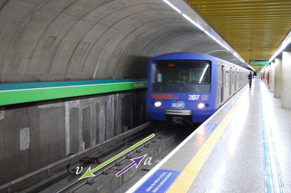
Acceleration is a vector in the same direction as the change in velocity, \(Δv\). Since velocity is a vector, it can change either in magnitude or in direction. Acceleration is therefore a change in either speed or direction, or both.
Keep in mind that although acceleration is in the direction of the change in velocity, it is not always in the direction of motion. When an object slows down, its acceleration is opposite to the direction of its motion. This is known as deceleration.
MISCONCEPTION ALERT: DECELERATION VS. NEGATIVE ACCELERATION
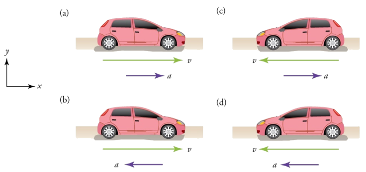
Deceleration always refers to acceleration in the direction opposite to the direction of the velocity. Deceleration always reduces speed. Negative acceleration, however, is acceleration in the negative direction in the chosen coordinate system. Negative acceleration may or may not be deceleration, and deceleration may or may not be considered negative acceleration. If acceleration has the same sign as the velocity, the object is speeding up. If acceleration has the opposite sign as the velocity, the object is slowing down. For example, consider Figure \(\PageIndex{2}\).
Example \(\PageIndex{1}\): Calculating Acceleration: A Racehorse Leaves the Gate
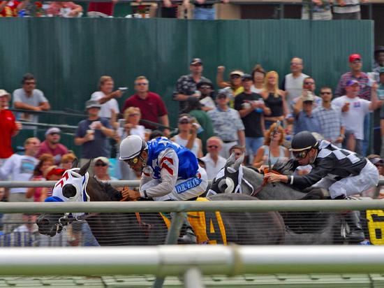
A racehorse coming out of the gate accelerates from rest to a velocity of 15.0 m/s due west in 1.80 s. What is its average acceleration?
Strategy
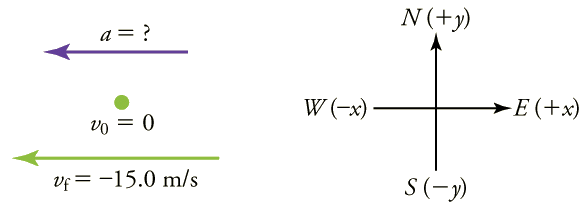
First we draw a sketch and assign a coordinate system to the problem. This is a simple problem, but it always helps to visualize it. Notice that we assign east as positive and west as negative. Thus, in this case, we have negative velocity.
We can solve this problem by identifying \(Δv\) and \(Δt\) from the given information and then calculating the average acceleration directly from the Equation \ref{averagea}:
\[\bar{a}=\dfrac{Δv}{Δt}=\dfrac{v_f−v_0}{t_f−t_0}. \nonumber\]
Solution
- Identify the knowns. \(v_0=0 , v_f=−15.0 m/s\) (the negative sign indicates direction toward the west), \( Δt=1.80 s\).
- Find the change in velocity. Since the horse is going from zero to \( −15.0 m/s\), its change in velocity equals its final velocity: \[Δv=v_f=−15.0\, m/s .\nonumber\]
- Plug in the known values ( \(Δv\) and \(Δt\) ) and solve for the unknown \(\bar{a}\).
\(\bar{a}=\frac{Δv}{Δt}=\frac{−15.0 m/s}{1.80 s}=−8.33 m/s^2\).
Discussion
The negative sign for acceleration indicates that acceleration is toward the west. An acceleration of \(8.33\, m/s^2\) due west means that the horse increases its velocity by 8.33 m/s due west each second, that is, 8.33 meters per second per second, which we write as \( 8.33\, m/s^2\). This is truly an average acceleration, because the ride is not smooth. We shall see later that an acceleration of this magnitude would require the rider to hang on with a force nearly equal to his weight.
Instantaneous Acceleration
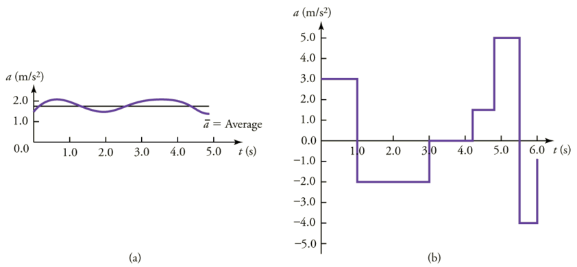
Instantaneous acceleration \( a\), or the acceleration at a specific instant in time, is obtained by the same process as discussed for instantaneous velocity in Time, Velocity, and Speed—that is, by considering an infinitesimally small interval of time. How do we find instantaneous acceleration using only algebra? The answer is that we choose an average acceleration that is representative of the motion. Figure \(\PageIndex{6}\) shows graphs of instantaneous acceleration versus time for two very different motions. In Figure \(\PageIndex{6a}\), the acceleration varies slightly and the average over the entire interval is nearly the same as the instantaneous acceleration at any time. In this case, we should treat this motion as if it had a constant acceleration equal to the average (in this case about \(1.8 m/s^2\)). In Figure \(\PageIndex{6b}\), the acceleration varies drastically over time. In such situations it is best to consider smaller time intervals and choose an average acceleration for each. For example, we could consider motion over the time intervals from 0 to 1.0 s and from 1.0 to 3.0 s as separate motions with accelerations of \( +3.0\, m/s^2\) and \( –2.0 \,m/s^2\), respectively.
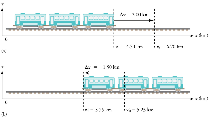
The next several examples consider the motion of the subway train shown in Figure \(\PageIndex{7}\). In Figure \(\PageIndex{7a}\) the shuttle moves to the right, and in Figure \(\PageIndex{7b}\) it moves to the left. The examples are designed to further illustrate aspects of motion and to illustrate some of the reasoning that goes into solving problems.
Example \(\PageIndex{2}\): Calculating Displacement - A Subway Train
What are the magnitude and sign of displacements for the motions of the subway train shown in parts (a) and (b) of Figure \(\PageIndex{7}\)?
Strategy
A drawing with a coordinate system is already provided, so we don’t need to make a sketch, but we should analyze it to make sure we understand what it is showing. Pay particular attention to the coordinate system. To find displacement, we use the equation \( Δx=x_f−x_0\). This is straightforward since the initial and final positions are given.
Solution
- Identify the knowns. In the figure we see that \(x_f=6.70\, km \) and \(x_0=4.70\, km\) for part (a), and \(x'_f=3.75\, km \) and \(x'_0=5.25\, km \) for part (b).
- Solve for displacement in part (a).\[\begin{align*} Δx &=x_f−x_0 \\[5pt] &=6.70\, km−4.70\, km \\[5pt] &=+2.00 \,km \end{align*}\]
- Solve for displacement in part (b).\[\begin{align*} Δx' &=x'_f−x'_0 \\[5pt] &=3.75\, km−5.25\, km \\[5pt] &=−1.50\, km \end{align*}\]
Discussion
The direction of the motion in (a) is to the right and therefore its displacement has a positive sign, whereas motion in (b) is to the left and thus has a negative sign.
Example \(\PageIndex{3}\): Comparing Distance Traveled with Displacement - A Subway Train
What are the distances traveled for the motions shown in parts (a) and (b) of the subway train in Figure \(\PageIndex{7}\)?Strategy
To answer this question, think about the definitions of distance and distance traveled, and how they are related to displacement. Distance between two positions is defined to be the magnitude of displacement, which was found in Example \(\PageIndex{2}\). Distance traveled is the total length of the path traveled between the two positions (see Section on Displacement). In the case of the subway train shown in Figure \(\PageIndex{7}\), the distance traveled is the same as the distance between the initial and final positions of the train.
Solution
1. The displacement for part (a) was +2.00 km. Therefore, the distance between the initial and final positions was 2.00 km, and the distance traveled was 2.00 km.
2. The displacement for part (b) was \( −1.5 km\). Therefore, the distance between the initial and final positions was 1.50 km, and the distance traveled was 1.50 km.
Discussion
Distance is a scalar. It has magnitude but no sign to indicate direction.
Example \(\PageIndex{4}\): Calculating Acceleration: A Subway Train Speeding Up
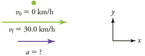
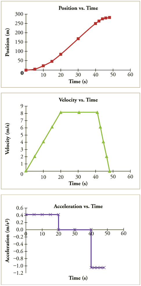
Suppose the train in Figure \(\PageIndex{7a}\) accelerates from rest to 30.0 km/h in the first 20.0 s of its motion. What is its average acceleration during that time interval?
Strategy
It is worth it at this point to make a simple sketch:
Solution
- Identify the knowns. \( v_0=0\) (the trains starts at rest), \( v_f=30.0 km/h \), and \(Δt=20.0 s \).
- Calculate \(Δv\). Since the train starts from rest, its change in velocity is \(Δv=+30.0 km/h \), where the plus sign means velocity to the right.
- Plug in known values and solve for the unknown, \(\bar{ a}\). \[\bar{a}=\dfrac{Δv}{Δt}=\dfrac{+30.0 km/h}{20.0 s}\nonumber\]
- Since the units are mixed (we have both hours and seconds for time), we need to convert everything into SI units of meters and seconds. (See Physical Quantities and Units for more guidance.) \[\bar{a}=\left(\dfrac{+30 km/h}{20.0 s}\right)\left(\dfrac{10^3m}{1 km}\right)\left(\dfrac{1h}{3600 s}\right)=0.417 m/s^2 \nonumber\]
Discussion
The plus sign means that acceleration is to the right. This is reasonable because the train starts from rest and ends up with a velocity to the right (also positive). So acceleration is in the same direction as the change in velocity, as is always the case.
Example \(\PageIndex{5}\): Calculate Acceleration
A Subway Train Slowing Down: Now suppose that at the end of its trip, the train in Figure \(\PageIndex{7a}\) slows to a stop from a speed of 30.0 km/h in 8.00 s. What is its average acceleration while stopping?
Strategy
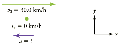
In this case, the train is decelerating and its acceleration is negative because it is toward the left. As in the previous example, we must find the change in velocity and the change in time and then solve for acceleration.
Solution
- Identify the knowns. \(v_0=30.0 km/h , v_f=0 km/h\) (the train is stopped, so its velocity is 0), and \(Δt=8.00 s \).
- Solve for the change in velocity, \(Δv\). \[Δv=v_f−v_0=0−30.0 km/h=−30.0 km/h \nonumber\]
- Plug in the knowns, \( Δv\) and \(Δt\), and solve for \(\bar{a}\). \[\bar{a}=\dfrac{Δv}{Δt}=\dfrac{−30.0 km/h}{8.00 s} \nonumber\]
- Convert the units to meters and seconds. \[\bar{a}=\dfrac{Δv}{Δt}=\left(\dfrac{−30.0 km/h}{8.00 s}\right)\left(\dfrac{10^3m}{1 km}\right)\left(\dfrac{1 h}{3600 s}\right)=−1.04 m/s^2. \nonumber\]
Discussion
The minus sign indicates that acceleration is to the left. This sign is reasonable because the train initially has a positive velocity in this problem, and a negative acceleration would oppose the motion. Again, acceleration is in the same direction as the change in velocity, which is negative here. This acceleration can be called a deceleration because it has a direction opposite to the velocity.
The graphs of position, velocity, and acceleration vs. time for the trains in Example \(\PageIndex{4}\) and \(\PageIndex{5}\) are displayed in Figure \(\PageIndex{10}\). (We have taken the velocity to remain constant from 20 to 40 s, after which the train decelerates.)
Example \(\PageIndex{6}\): Calculating Average Velocity: The Subway Train
What is the average velocity of the train in part b of Example \(\PageIndex{2}\), and shown again below, if it takes 5.00 min to make its trip?

Strategy
Average velocity is displacement divided by time. It will be negative here, since the train moves to the left and has a negative displacement.
Solution
- Identify the knowns. \[ x'_f=3.75 km,\, x'_0=5.25 km,\, Δt=5.00 min. \nonumber\]
- Determine displacement, \(Δx'\). We found \( Δx'\) to be \( −1.5 km\) in Example \(\PageIndex{7}\).
- Solve for average velocity. \[\bar{v}=\dfrac{Δx'}{Δt}=\dfrac{−1.50 km}{5.00 min} \nonumber\]
- Convert units. \[\bar{v}=\dfrac{Δx'}{Δt}=(\dfrac{−1.50 km}{5.00 min})(\dfrac{60 min}{1 }h)=−18.0 km/h \nonumber\]
Discussion
The negative velocity indicates motion to the left.
Example \(\PageIndex{7}\): Calculating Deceleration: The Subway Train
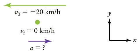
Finally, suppose the train in Figure \(\PageIndex{7}\) slows to a stop from a velocity of 20.0 km/h in 10.0 s. What is its average acceleration?
Strategy
Once again, let’s draw a sketch:
Solution
- Identify the knowns. \(v_0=−20\, km/h\), \(v_f=0\, km/h\), \(Δt=10.0\, s\).
- Calculate \(Δv\). The change in velocity here is actually positive, since \[Δv=v_f−v_0=0−(−20\, km/h)=+20\, km/h. \nonumber\]
- Solve for \(\bar{ a}\). \[\bar{a}=\dfrac{Δv}{Δt}=\dfrac{+20.0\, km/h}{10.0\, s} \nonumber\]
- Convert units. \[\bar{a}=\left(\dfrac{+20.0 \,km/h}{10.0\, s}\right)\left(\dfrac{10^3\,m}{1\, km}\right)\left(\dfrac{1\, h}{3600 \,s}\right)=+0.556\, m/^s2 \nonumber\]
Discussion
The plus sign means that acceleration is to the right. This is reasonable because the train initially has a negative velocity (to the left) in this problem and a positive acceleration opposes the motion (and so it is to the right). Again, acceleration is in the same direction as the change in velocity, which is positive here. As in Example \(\PageIndex{5}\), this acceleration can be called a deceleration since it is in the direction opposite to the velocity.
Sign and Direction
Perhaps the most important thing to note about these examples is the signs of the answers. In our chosen coordinate system, plus means the quantity is to the right and minus means it is to the left. This is easy to imagine for displacement and velocity. But it is a little less obvious for acceleration. Most people interpret negative acceleration as the slowing of an object. This was not the case in Example \(\PageIndex{5}\), where a positive acceleration slowed a negative velocity. The crucial distinction was that the acceleration was in the opposite direction from the velocity. In fact, a negative acceleration will increase a negative velocity. For example, the train moving to the left in Figure Figure \(\PageIndex{11}\) is sped up by an acceleration to the left. In that case, both v and a are negative. The plus and minus signs give the directions of the accelerations. If acceleration has the same sign as the velocity, the object is speeding up. If acceleration has the opposite sign as the velocity, the object is slowing down.
Exercise \(\PageIndex{1}\)
An airplane lands on a runway traveling east. Describe its acceleration.
- Answer
-
If we take east to be positive, then the airplane has negative acceleration, as it is accelerating toward the west. It is also decelerating: its acceleration is opposite in direction to its velocity.
PHET EXPLORATIONS: MOVING MAN SIMULATION
Learn about position, velocity, and acceleration graphs with the PhET Moving Man simulation. Move the little man back and forth with the mouse and plot his motion. Set the position, velocity, or acceleration and let the simulation move the man for you.
Summary
- Acceleration is the rate at which velocity changes. In symbols, average acceleration \(\bar{ a}\) is \(\bar{a}=\dfrac{Δv}{Δt}=\dfrac{v_f−v_0}{t_f−t_0}\).
- The SI unit for acceleration is 2 .
- Acceleration is a vector, and thus has a both a magnitude and direction.
- Acceleration can be caused by either a change in the magnitude or the direction of the velocity.
- Instantaneous acceleration is the acceleration at a specific instant in time.
- Deceleration is an acceleration with a direction opposite to that of the velocity.
Glossary
- acceleration
- the rate of change in velocity; the change in velocity over time
- average acceleration
- the change in velocity divided by the time over which it changes
- instantaneous acceleration
- acceleration at a specific point in time
- deceleration
- acceleration in the direction opposite to velocity; acceleration that results in a decrease in velocity


