
12.5: Uncertainty Principle
- Page ID
- 46245

Learning Objectives
- Describe the position-momentum uncertainty principle.
- Explain the relationship between wave-particle dual nature and the uncertainty principle
Probability Wave
The de Broglie wavelength assigns a wave nature to everything, even to the things we are used to thinking of as particles, such as an electron. So, what kind of waves are they? As far as we know, there are not smaller parts that electron can be broken into that can be oscillating. Furthermore, when we measure the position of the electron, each time, we find the electron at some definite location, as we would expect for a particle. So, what kind of a wave is electron?
Figure \(\PageIndex{1}\) illustrates a result of electron interference experiment. Each dot represents the location where an electron was detected, and you see that with few electrons, dots appear spread out more or less randomly, and it is not obvious if there is any location where constructive interference or destructive interference is occurring. But as you continue to collect more data (more electrons detected), a pattern begins to emerge, where there are locations where electrons are mysteriously never detected. Those are the locations where electron waves—whatever they are—are destructively interfering.
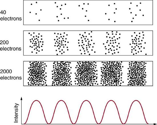
After de Broglie proposed the wave nature of matter, many physicists, including Schrödinger and Heisenberg, explored the consequences. The Schrödinger equation is the wave equation (a type of differential equation) which describes the behavior of these matter waves. This still doesn't quite answer what kind of a wave an electron is—and we won't really answer it, in a similar way as how we can say that a photon is an electromagnetic wave—so for now, we will give this wave a name: "probability wave." The wave function which corresponds to the wave nature of electron describes the probability of detecting the particle at a particular location and time. And this wave nature becomes evident experimentally only in the statistical sense. That is, after compiling enough data, you get a distribution of the particle locations, and you can calculate a certain probability of finding the particle at a given location. This overall pattern is called a probability distribution. Those who developed quantum mechanics devised equations (of which the Schrödinger equation is one example) that predicted the probability distribution in various circumstances.
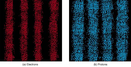
The most disquieting aspect of quantum mechanics is that the nature, at its most fundamental level, can only be described probabilistically. In Figure \(\PageIndex{1}\) and Figure \(\PageIndex{2}\) above, for each dot representing an electron or a photon, the experimental setup was identically. But with this identical set up, each electron (or each photon) ends up taking different paths, ending at the location represented by the dot. In classical mechanics, we would say this was because of our incomplete knowledge of the setup (we don't know the precise way an electron bounces off from the barriers on its way to the screen where it is detected). In quantum mechanics, even in theory—assuming the most complete knowledge theoretically possible—we can only describe probability of finding the electron at one location, and the theory does not allow for prediction of individual electron paths. This aspect disturbed many physicists working on quantum mechanics, including Albert Einstein, who exclaimed, incorrectly, "God does not play dice."
Heisenberg Uncertainty Principle
If the theory does not allow prediction of individual electron path, could we simply measure the location of the electron as it travels toward the screen? When such experiment was done, the experimenters found more than what paths the electrons took to result in the interference pattern. They found that the interference pattern itself was gone, with the constructive and destructive interference fringes smeared out!
The answer here is fundamentally important—measurement affects the system being observed, even in theory. Even with the most sensitive of measurement devices, by the very act of measuring a physical observable (for example, particle position), you alter the state of the system. So in some cases it is impossible to measure two physical quantities to exact precision at the same time (you can measure one to exact precision and then measure the other to exact precision, but those will be two exact-precision measurements for two different particle states).
Here is an example to consider to illuminate why this is so. Suppose you want to measure the position of a moving electron. To "see" where the electron is, you need to scatter another particle (either light—photon—or another particle) off of it. But these probes will have a momentum, and by scattering from the electron, they change the momentum of the electron. So, by measuring the position of the electron, you change its momentum (and it's this change of momentum that leads to the interference pattern being smeared out). There is a limit to absolute knowledge, even in principle.
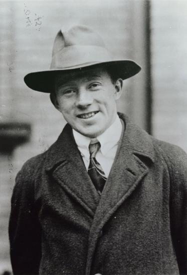
It was Werner Heisenberg who first stated this limit to knowledge in 1929 as a result of his work on quantum mechanics and the wave characteristics of all particles. (See Figure \(\PageIndex{3}\)). Specifically, consider simultaneously measuring the position and momentum of an electron (it could be any particle). There is an uncertainty in position \(\Delta x\) that is approximately equal to the wavelength of the particle. That is,
\[\Delta x \approx \lambda. \nonumber \]
Unless the electron wave function is spread out as much as its average wavelength, the meaning of wavelength itself becomes unclear (what is the wavelength of something that exists only at one point?). To detect the position of the particle, we must interact with it, such as having it collide with a detector. In the collision, the particle will lose momentum. This change in momentum could be anywhere from close to zero to the total momentum of the particle, \(p=h / \lambda\). It is not possible to tell how much momentum will be transferred to a detector, and so there is an uncertainty in momentum \(\Delta p\), too. In fact, with these subatomic particles, the uncertainty in momentum may be as large as the momentum itself, which in equation form means (using the de Broglie relationship) that
\[\Delta p \approx p=\frac{h}{\lambda}. \nonumber \]
The uncertainty in position can be reduced by using a shorter-wavelength electron, since \(\Delta x \approx \lambda\). But shortening the wavelength increases the uncertainty in momentum, since \(\Delta p \approx h / \lambda\). Conversely, the uncertainty in momentum can be reduced by using a longer-wavelength electron, but this increases the uncertainty in position. Mathematically, you can express this trade-off by multiplying the uncertainties. The wavelength cancels, leaving
\[\Delta x \Delta p \approx h. \nonumber \]
So if one uncertainty is reduced, the other must increase so that their product is \(\approx h\).
With the use of advanced mathematics (with uncertainties being precisely defined using statistical concepts such as standard deviation), Heisenberg showed that the best that can be done in a simultaneous measurement of position and momentum is
\[\Delta x \Delta p \geq \frac{h}{4 \pi}. \nonumber \]
This is known as the Heisenberg uncertainty principle. It is impossible to measure position \(x\) and momentum \(p\) simultaneously with uncertainties \(\Delta x\) and \(\Delta p\) that multiply to be less than \(h / 4 \pi\). Neither uncertainty can be zero. Neither uncertainty can become small without the other becoming large.
A small wavelength allows accurate position measurement, but it increases the momentum of the probe to the point that it further disturbs the momentum of a system being measured. For example, if an electron is scattered from an atom and has a wavelength small enough to detect the position of electrons in the atom, its momentum can knock the electrons from their orbits in a manner that loses information about their original motion. It is therefore impossible to follow an electron in its orbit around an atom. If you measure the electron’s position, you will find it in a definite location at that moment, but with the uncertain amount of momentum transferred, you will not know where that electron will be in the next moment.
Example \(\PageIndex{1}\): Heisenberg Uncertainty Principle in Position and Momentum for an Atom
(a) If the position of an electron in an atom is measured to an accuracy of 0.0100 nm, what is the electron’s uncertainty in velocity? (b) If the electron has this velocity, what is its kinetic energy in eV?
Strategy
The uncertainty in position is the accuracy of the measurement, or \(\Delta x=0.0100 \mathrm{~nm}\). Thus the smallest uncertainty in momentum \(\Delta p\) can be calculated using \(\Delta x \Delta p \geq h / 4 \pi\). Once the uncertainty in momentum \(\Delta p\) is found, the uncertainty in velocity can be found from \(\Delta p=m \Delta v\).
Solution for (a)
Using the equals sign in the uncertainty principle to express the minimum uncertainty, we have
\[\Delta x \Delta p=\frac{h}{4 \pi}. \nonumber\]
Solving for \(\Delta p\) and substituting known values gives
\[\Delta p=\frac{h}{4 \pi \Delta x}=\frac{6.63 \times 10^{-34} \mathrm{~J} \cdot \mathrm{s}}{4 \pi\left(1.00 \times 10^{-11} \mathrm{~m}\right)}=5.28 \times 10^{-24} \mathrm{~kg} \cdot \mathrm{m} / \mathrm{s}. \nonumber\]
Thus,
\[\Delta p=5.28 \times 10^{-24} \mathrm{~kg} \cdot \mathrm{m} / \mathrm{s}=m \Delta v. \nonumber\]
Solving for \(\Delta v\) and substituting the mass of an electron gives
\[\Delta v=\frac{\Delta p}{m}=\frac{5.28 \times 10^{-24} \mathrm{~kg} \cdot \mathrm{m} / \mathrm{s}}{9.11 \times 10^{-31} \mathrm{~kg}}=5.79 \times 10^{6} \mathrm{~m} / \mathrm{s}. \nonumber\]
Solution for (b)
Although large, this velocity is not highly relativistic, and so the electron’s kinetic energy is
\[\begin{aligned}
\mathrm{KE}_{e} &=\frac{1}{2} m v^{2} \\
&=\frac{1}{2}\left(9.11 \times 10^{-31} \mathrm{~kg}\right)\left(5.79 \times 10^{6} \mathrm{~m} / \mathrm{s}\right)^{2} \\
&=\left(1.53 \times 10^{-17} \mathrm{~J}\right)\left(\frac{1 \mathrm{eV}}{1.60 \times 10^{-19} \mathrm{~J}}\right)=95.5 ~\mathrm{eV}.
\end{aligned} \nonumber\]
Discussion
Since atoms are roughly 0.1 nm in size, knowing the position of an electron to 0.0100 nm localizes it reasonably well inside the atom. This would be like being able to see details one-tenth the size of the atom. But the consequent uncertainty in velocity is large. You certainly could not follow it very well if its velocity is so uncertain. To get a further idea of how large the uncertainty in velocity is, we assumed the velocity of the electron was equal to its uncertainty and found this gave a kinetic energy of 95.5 eV. This is significantly greater than the typical energy difference between levels in atoms, so that it is impossible to get a meaningful energy for the electron if we know its position even moderately well.
Why don’t we notice Heisenberg’s uncertainty principle in everyday life? The answer is that Planck’s constant is very small. Thus the lower limit in the uncertainty of measuring the position and momentum of large objects is negligible. We can detect sunlight reflected from Jupiter and follow the planet in its orbit around the Sun. The reflected sunlight alters the momentum of Jupiter and creates an uncertainty in its momentum, but this is totally negligible compared with Jupiter’s huge momentum. The correspondence principle tells us that the predictions of quantum mechanics become indistinguishable from classical physics for large objects, which is the case here.
Finally, note that in the discussion of particles and waves, we have stated that individual measurements produce precise or particle-like results. A definite position is determined each time we observe an electron, for example (represented as dots). But repeated measurements produce a spread in values consistent with wave characteristics, illustrating the underlying probability density. The great theoretical physicist Richard Feynman (1918–1988) commented, “What there are, are particles.” When you observe enough of them, they distribute themselves as you would expect for a wave phenomenon. However, what there are as they travel we cannot tell because, when we do try to measure, we affect the traveling.
Section Summary
- Matter is found to have the same interference characteristics as any other wave.
- There is now a probability distribution for the location of a particle rather than a definite position.
- Another consequence of the wave character of all particles is the Heisenberg uncertainty principle, which limits the precision with which certain physical quantities can be known simultaneously. For position and momentum, the uncertainty principle is \(\Delta x \Delta p \geq \frac{h}{4 \pi}\), where \(\Delta x\) is the uncertainty in position and \(\Delta p\) is the uncertainty in momentum.
- These small limits are fundamentally important on the quantum-mechanical scale.
Glossary
- Heisenberg’s uncertainty principle
- a fundamental limit to the precision with which pairs of quantities (momentum and position, and energy and time) can be measured
- uncertainty in momentum
- lack of precision or lack of knowledge of precise results in measurements of momentum
- uncertainty in position
- lack of precision or lack of knowledge of precise results in measurements of position
- probability wave
- the description of wave characteristic of matter, as revealed by probability distribution experimentally
- probability distribution
- the overall spatial distribution of probabilities to find a particle at a given location