1.2: Maxwell’s Equations

In principle, given the positions of a collection of charged particles at each instant of time one could calculate the electric and magnetic fields at each point in space and at each time from Equations (1.1.9) and (1.1.10). For ordinary matter this is clearly an impossible task. Even a small volume of a solid or a liquid contains enormous numbers of atoms. A cube one micron on a side (10⁻⁶m × 10⁻⁶m × 10⁻⁶m) contains ∼ 10¹¹ atoms, for example. Each atom consists of a positively charged nucleus surrounded by many negatively charged electrons, all of which are in motion and which will, therefore, generate electric and magnetic fields that fluctuate rapidly both in space and in time. For most purposes one does not wish to know in great detail the space and time variation of the fields. One usually wishes to know about the space and time averaged electric and magnetic fields. For example, the magnitude and direction of \(\vec E\) averaged over a time interval that is determined by the instrument used to measure the field. Typically this might be of order 10⁻⁶ seconds or more; a time that is very long compared with the time required for an electron to complete an orbit around the atomic nucleus in an atom (10⁻¹⁶ to 10⁻²¹ seconds). Moreover, one is usually interested in the value of these fields averaged over a volume that is small compared with a cube ∼ 10⁻⁶ meters on a side but large compared with atomic dimensions, ∼ 10⁻¹⁰ meters in diameter. In 1864 J.C.Maxwell proposed a system of differential equations that can be used for calculating electric and magnetic field distributions, and that automatically provide the space and time averaged fields that are of practical interest. These Maxwell’s Equations for a macroscopic medium are as follows:

\[ \begin{align} & \operatorname{curl} \vec{\mathrm{E}}=-\frac{\partial \vec{\mathrm{B}}}{\partial t} \label{1.13} \\& \operatorname{div} \vec{\mathrm{B}}=0 \label{1.14} \\& \operatorname{curl} \vec{\mathrm{B}}=\mu_{0}\left(\vec{\mathrm{J}}_{f}+\operatorname{curl} \vec{\mathrm{M}}+\frac{\partial \vec{\mathrm{P}}}{\partial t}\right)+\epsilon_{0} \mu_{0} \frac{\partial \vec{\mathrm{E}}}{\partial t} \label{1.15} \\& \operatorname{div} \vec{\mathrm{E}}=\frac{1}{\epsilon_{0}}\left(\rho_{f}-\operatorname{div} \vec{\mathrm{P}}\right) \label{1.16} \end{align}\]

where \(\epsilon_{0} \mu_{0}=1 / c^{2}\) and c is the velocity of light in vacuum. These equations underlie all of electrical engineering and much of physics and chemistry. They should be committed to memory. In large part, this book is devoted to working out the consequences of Maxwell’s equations for special cases that provide the required background and guidance for solving practical problems in electricity and magnetism. In Equations (1.2.13 to 1.2.16) \(\epsilon_{0}\) is the permativity of free space; it has already been introduced in connection with Coulomb’s law, Equation (1.1.3). The constant µ₀ is called the permeability of free space. It has the defined value

\[\mu_{0}=4 \pi \times 10^{-7} \quad \text { Henries / } m. \label{1.17}\]

Maxwell’s equations as written above contain four new quantities which must be defined: they are

(1) \(\vec J_f\), the current density due to the charges which are free to move in space, in units of Amp`eres/m² ;

(2) ρ_f, the net density of charges in the material, in units of Coulombs/m³ ;

(3) \(\vec M\), the density of magnetic dipoles per unit volume in units of Amps/m;

(4) \(\vec P\), the density of electric dipoles per unit volume in units of Coulombs/m² . In Maxwell’s scheme these four quantities become the sources that generate the electric and magnetic fields. They are related to the space and time averages of the position and velocities of the microscopic charges that make up matter.

1.2.1 Definition of the Free Charge Density, ρ_f.

Construct a small volume element, ∆V , around the particular point in space specified by the position vector \(\vec r\). Add up all the charges contained in ∆V at a particular instant; let this amount of charge be ∆Q(t). Average ∆Q(t) over a time interval short compared with the measuring time of interest, but long compared with times characteristic of the motion of electrons around the atomic nuclei; let the resulting time averaged charge be < ∆Q(t) >. Then the free charge density is defined to be

\[\rho_{f}(\vec{r}, t)=\frac{<\Delta Q(t)>}{\Delta V} \quad \text { Coulombs } / m^{3}. \label{1.18}\]

The dimensions of the volume element ∆V is rather vague; it will depend upon the scale of the spatial variation that is of interest for a particular problem. It should be large compared with atomic dimensions but small compared with the distance over which ρ_f changes appreciably.

1.2.2 Definition of the Free Current Density, \(\vec J_f\).

The free charge density, \(\rho(\vec{\mathrm{r}}, t)\), will in general change with time as charge flows from one place to the other; one need only think of charge flowing along a wire. The rate at which charge flows across an element of area is described by the current density, \(\vec{\mathrm{J}}_{f} ( \vec{\mathrm{r}}, t)\). It is a vector because the charge flow is associated with a direction. The components of the current density vector can be measured by counting the rate of charge flow across a small area ∆A located at the position specified by \(\vec r\), and whose normal is oriented parallel with one of the co-ordinate axes; parallel with the x-axis, for example (see Figure (1.2.4)).

Figure \(\PageIndex{4}\): The x-component of the current density caused by a moving charge distribution. The charge labelled Q is representative of all charges passing through the x-oriented element of area, ∆A per unit time.

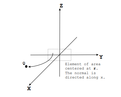
Now at time t measure the net amount of charge, < ∆Q >, that has passed through ∆A_x in a small time interval, ∆t: positive charge that flows in the direction from +x to -x is counted as a negative contribution; negative charge that flows from -x to +x also makes a negative contribution. The x-component of the current density is given by

\[\left.\vec{\mathrm{J}_{f}}\right|_{x}=\frac{<\Delta Q>}{\Delta t \Delta A_{x}} \quad A m p s / m^{2}. \label{1.19}\]

The other two components of \(\vec J_f\) are defined in a similar manner. The time interval ∆t, and the dimensions of the elements of area, ∆A_x, ∆A_y, and ∆A_z are supposed to be chosen so that they are large compared with atomic times and atomic dimensions, but small compared with the time and length scales appropriate for a particular problem. Free charge density can be visualized as a kind of fluid flowing from place to place with a certain velocity. In terms of this velocity the free current density is given by

\[\vec{\mathrm{J}}_{f}(\vec{\mathrm{r}}, t)=\rho_{f}(\vec{\mathrm{r}}, t) \vec{\mathrm{v}}(\vec{r}, t). \label{1.20}\]

In the process of charge flow electrical charge can neither be created nor destroyed. Because charge is conserved, it follows that the rate at which charge is carried into a volume must be related to the rate at which the net charge in the volume increases with time. The mathematical expression of this charge conservation law is

\[\frac{\partial \rho_{f}(\vec{\mathbf{r}}, t)}{\partial t}=-\operatorname{div} \vec{\mathbf{J}}_{f}(\vec{\mathbf{r}}, t). \label{1.21}\]

1.2.3 Point Dipoles.

In order to discuss the definitions of the two vector functions \(\vec{\mathrm{P}}(\vec{\mathrm{r}}, t)\) and \(\vec{\mathrm{M}}(\vec{\mathrm{r}}, t)\) it is first necessary to discuss the concepts of a point electric dipole and a point magnetic dipole.

The Point Electric Dipole.

Most atoms in a substance are electrically neutral, ie. the charge on the nucleus is compensated by the electrons moving around that nucleus. When examined from a distance that is long compared with atomic dimensions (∼ 10⁻¹⁰m) the neutral atom produces no substantial electric or magnetic field. However, if, on average, the centroid of the negative charge distribution is displaced from the position of the nucleus the Coulomb field of the nucleus will no longer cancel the Coulomb field from the electrons. To fix ideas, think of a stationary hydrogen atom consisting of a proton and an electron. The electron moves so fast that on a human time scale its charge appears to be located in a spherical cloud which is tightly distributed around the nucleus (see Figure 1.2.5).

In the absence of an external electric field the centroid of the electronic charge distribution will coincide with the position of the nucleus. Under these circumstances the time-averaged Coulomb fields of the nucleus and the electron cancel each other when observed from distances that are large

Figure \(\PageIndex{5}\): Upper figure: Sketch of a hydrogen atom in zero applied electric field. The nuclear charge is Q = 1.6 × 10⁻¹⁹ Coulombs. The time-averaged electron charge, -Q, is distributed in a spherically symmetric cloud around the nucleus having a radius of approximately 5 × 10⁻¹¹ m. Lower figure: Sketch of a hydrogen atom subjected to a uniform electric field E₀ . The displacement of the centroid of the electron charge density relative to the nucleus has been exaggerated for the sake of clarity.

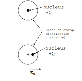
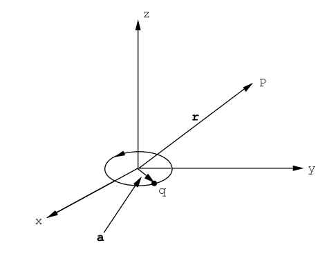
compared with 10⁻¹⁰m. If the atom is subjected to an external electric field the nucleus is pulled one way and the centroid of the electron cloud is pulled the other way (Equation (1.1.1)): there is an effective charge separation (see Figure 1.2.5). The Coulomb fields due to the nucleus and the electron no longer exactly cancel. Let us use the law of superposition to calculate the field that arises when two point charges no longer coincide; refer to Figure (1.2.6). The electric field at the point of observation, P, due to the positive charge is given by

\[\vec{\mathrm{E}}_{+}=\frac{q}{4 \pi \epsilon_{0}}\left(\frac{\vec{\mathrm{r}}}{\mathrm{r}^{3}}\right). \nonumber \]

The electric field at P due to the negative charge is given by

\[\vec{\mathrm{E}}_{-}=-\frac{q}{4 \pi \epsilon_{0}}\left(\frac{\vec{\mathrm{r}}+\vec{\mathrm{d}}}{\left(|\vec{\mathrm{r}}+\vec{\mathrm{d}}|^{3}\right.}\right). \nonumber \]

Figure \(\PageIndex{6}\): Two charges equal in magnitude but opposite in sign are separated by the vector distance \(\vec d\). By definition the dipole moment of this pair of charges is \(\vec{\mathrm{p}}=q \vec{\mathrm{d}}\) where \(\vec d\) is the vector directed from the negative to the positive charge. \(\hat{\mathrm{u}}_{\mathrm{x}}, \hat{\mathrm{u}}_{\mathrm{y}}, \text { and } \hat{\mathrm{u}}_{\mathrm{z}}\) are unit vectors directed along the x,y, and z axes.

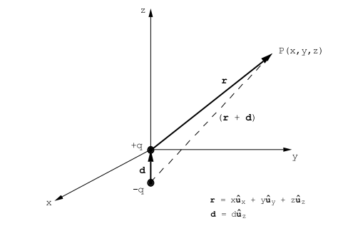
Referring to Figure 1.2.6 one has

\[\vec{\mathrm{r}}=x \hat{\mathrm{u}}_{x}+y \hat{\mathrm{u}}_{y}+z \hat{\mathrm{u}}_{z}, \nonumber\]

and

\[\mathrm{r}=\sqrt{x^{2}+y^{2}+z^{2}}. \nonumber\]

For \(\vec d\) oriented along the z-axis as shown in Figure 1.2.6,

\[(\vec{\mathrm{r}}+\vec{\mathrm{d}})=x \hat{\mathrm{u}}_{x}+y \hat{\mathrm{u}}_{y}+(z+d) \hat{\mathrm{u}}_{z} \nonumber\]

so that

\[ \left.|\vec{r}+\vec{d}|=\left[x^{2}+y^{2}+(z+d)^{2}\right)\right]^{1 / 2} \nonumber \]

or

\[|\vec{\mathrm{r}}+\vec{\mathrm{d}}|=\left[x^{2}+y^{2}+z^{2}+2 z d+d^{2}\right]^{1 / 2}. \nonumber\]

Upon dividing out r² this gives

\[|\vec{\mathrm{r}}+\vec{\mathrm{d}}|=r\left[1+\left(\frac{2 z d+d^{2}}{r^{2}}\right)\right]^{1 / 2}. \nonumber \]

From this expression one has

\[\frac{1}{|\vec{\mathrm{r}}+\vec{\mathrm{d}}|^{3}}=\frac{1}{r^{3}}\left[1+\frac{\left(2 z d+d^{2}\right)}{r^{2}}\right]^{-3 / 2}. \nonumber \]

This is so far exact. Now make use of the fact that (d/r) is very small and use the binomial theorem to expand the radical. It is sufficient to keep only terms linear in (d/r). The result is

\[\frac{1}{|\vec{\mathrm{r}}+\vec{\mathrm{d}}|^{3}}=\frac{1}{r^{3}}-\frac{3 z d}{r^{5}}. \nonumber\]

Use this result to calculate the total electric field at the point of observation, P, correct to terms of order (d/r). The terms proportional to

\[\left(\frac{1}{r^{2}}\right) \nonumber\]

cancel leaving the field

\[\vec{\mathrm{E}_{d}}=\vec{\mathrm{E}_{+}}+\vec{\mathrm{E}_{-}}=\frac{1}{4 \pi \epsilon_{0}}\left(\frac{(3 z q d) \vec{\mathrm{r}}}{r^{5}}-\frac{q \vec{\mathrm{d}}}{r^{3}}\right). \nonumber\]

By definition the dipole moment of the pair of point charges is given by \(\vec{\mathrm{p}}=q \vec{\mathrm{d}}\). Moreover, \(zqd=\vec r \cdot \vec p \), ie. it is equal to the scalar product of the dipole moment and the position vector \(\vec r\). Finally, the expression for the electric field generated by a stationary point dipole can be written

\[\vec{\mathrm{E}_{d}}=\frac{1}{4 \pi \epsilon_{0}}\left(\frac{3(\vec{\mathrm{p}} \cdot \vec{\mathrm{r}}) \vec{\mathrm{r}}}{r^{5}}-\frac{\vec{\mathrm{p}}}{r^{3}}\right).\label{1.22}\]

Although this expression has been obtained for the particular case in which \(\vec p\) is oriented along the z-axis, the result stated in Equation (\ref{1.22}) is perfectly general and is valid for any orientation of the dipole moment \(\vec p\).

Formula \ref{1.22} is so fundamental that it should be committed to memory along with Coulomb’s law. The field distribution around a point dipole is illustrated in Figure 1.2.7. The magnetic field generated by a stationary point dipole is zero; magnetic fields are generated by charges moving with respect to the observer.

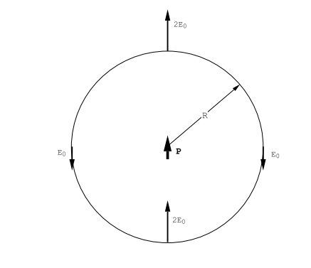
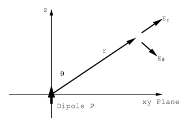
It is useful to write the dipole electric field in terms of it’s components with respect to a spherical polar co-ordinate system in which the dipole is aligned along the z-axis, see Figure (1.2.8). These components are

\[\mathrm{E}_{\mathrm{r}}=\frac{2 p}{4 \pi \epsilon_{0}} \frac{\cos (\theta)}{r^{3}}\label{1.23}\]

\[\mathrm{E}_{\theta}=\frac{p}{4 \pi \epsilon_{0}} \frac{\sin (\theta)}{r^{3}} \label{1.24}\]

The Point Magnetic Dipole.

Atoms and molecules often carry a magnetic moment. These magnetic moments can arise as a result of the motion of electrons around the nucleus of an atom or around the nuclei in a molecule (see below). In addition,

Figure \(\PageIndex{7}\): The electric field intensity at various positions around an electric point dipole, \(\vec P\). The electric field distribution is cylindrically symmetric around the dipole as axis.

electrons and nuclei carry intrinsic point magnetic moments that are related to their intrinsic angular momentum (spin). Atomic or molecular magnetic moments generate magnetic fields. When these magnetic fields are observed at distances from the atom or molecule that are much larger than atomic or molecular dimensions, and when these fields are averaged over times long compared with atomic or molecular orbital times, the resulting time averaged field can be described by

\[\vec{\mathrm{B}}=\frac{\mu_{0}}{4 \pi}\left(\frac{3(\vec{\mathrm{m}} \cdot \vec{\mathrm{r}}) \vec{\mathrm{r}}}{r^{5}}-\frac{\vec{\mathrm{m}}}{r^{3}}\right). \label{1.25}\]

where µ₀ is the constant of Equation (\ref{1.17}) and \(\vec m\) is the magnetic moment. In addition to the magnetic field created by a magnetic moment, the atom or molecule, if charged, will generate an electric field given by Coulomb’s law, Equation (1.1.3).

Figure \(\PageIndex{8}\): The electric field generated by a dipole oriented along the z-axis and expressed as spherical polar components.

The generation of a magnetic field due to the orbital motion of a charged particle can be understood using the simple model illustrated in Figure (1.1.9). Let a spinless charged particle, charge= q Coulombs, revolve in a circular orbit of radius a meters with the speed v meters/sec, where \(\frac{v}{c} << 1 \). One can use Equation (1.1.7) to calculate the electric and magnetic fields that would be measured by an observer whose distance from the center of the current loop is much greater than the orbit radius a. It can be shown that the time averaged electric field is given by coulomb’s law

\[\vec{\mathrm{E}}=\frac{q}{4 \pi \epsilon_{0}}\left(\frac{\vec{r}}{r^{3}}\right) \quad \text { Volts } / \mathrm{m}. \nonumber\]

This result is obtained by using a binomial expansion in the small quantity a/r and keeping only the lowest order terms; the lowest order correction term upon taking the time average is proportional to (a/r)² , see problem (1.8). The magnetic field can be calculated using Equation (1.1.7). The velocity of the particle is proportional to the orbit radius, and therefore when the time averages are worked out the lowest order non-vanishing term is proportional to (a/r)² ; see problem (1.8). The time-averaged magnetic field turns out to be given by Equation (\ref{1.25}). Notice that this expression has exactly the same form as Equation (\ref{1.22}) for the electric field distribution around an electric dipole

Figure \(\PageIndex{9}\): A particle carrying a charge of q Coulombs and following a circular orbit of radius a meters with the speed v meters/sec generates a magnetic dipole moment \(|\vec{\mathrm{m}}|=\text { qav } / 2 \mathrm{Amp}-m^{2}\).

moment \(\vec p\). Here the vector m is called the orbital magnetic dipole moment associated with the current loop, and is given by

\[\vec{\mathrm{m}}=\frac{q a^{2}}{2}\left(\frac{d \phi}{d t}\right) \hat{\mathrm{u}}_{z} \quad \text { Coulomb }-\text { meters }^{2} / \text { sec. } \label{1.26}\]

Note that \(|\vec{\mathrm{m}}|=\mathrm{IA}\) where \(\mathrm{I}=\mathrm{qv} / 2 \pi a\) is the current in the loop, and \(A=\pi a^{2}\) is the area of the loop. Since the speed of the particle is given by \(v=a(\mathrm{d} \phi / d t)\), the magnitude of the magnetic moment can also be written in terms of the angular momentum of the circulating charge:

\[ |\vec{\mathrm{m}}|=\frac{q a \mathrm{v}}{2}=\left(\frac{q}{2 m_{p}}\right)\left(m_{p} a v\right). \nonumber\]

where the mass of the charged particle is m_p and it carries an angular momentum \(\mathrm{L}=\mathrm{m}_{p} a \mathrm{v}\). Thus the angular momentum \(\vec m\) is related to the particle angular momentum \(vec L\) by the relation

\[\vec{\mathrm{m}}=\left(\frac{q}{2 m_{p}}\right) \vec{\mathrm{L}}. \label{1.27}\]

For an electron q= - 1.60 × 10⁻¹⁹ Coulombs = - |e| so that the magnetic moment and the angular momentum are oppositely directed. The angular momentum is quantized in units of \(\hbar\), therefore the magnetic moment of an orbiting particle is also quantized. The quantum of magnetization for an orbiting electron is called the Bohr magneton, µ_B. It has the value

\[ \mu_{B}=\frac{e \hbar}{2 m_{e}}=9.27 \times 10^{-24} \quad \text { Coulomb }-m^{2} / \mathrm{sec}. \nonumber\]

(The units of µ_B can also be expressed as Amp-m² or as Joules/Tesla).

In addition to their orbital angular momentum, charged particles possess intrinsic or spin angular momentum, \(\vec S\). There is also a magnetic moment associated with the spin. The magnetic moment due to spin is usually written

\[\vec{\mathrm{m}}_{s}=g\left(\frac{q}{2 m_{p}}\right) \vec{\mathrm{s}}. \label{1.28}\]

For an electron q = −|e|, and g = 2.00. The spin of an electron has the magnitude |\(\vec S\)| = \(\hbar\)/2; consequently, the intrinsic magnetic moment carried an electron due to its spin is just 1 Bohr magneton, µ_B. The total magnetic moment generated by an orbiting particle that carries a spin moment is given by the vector sum of its orbital and spin magnetic moments. The total magnetic moment associated with an atom is the vector sum of the orbital and spin moments carried by all of its constituent particles, including the nucleus. The magnetic field generated by a stationary atom at distances large compared with the atomic radius is given by Equation (\ref{1.25}) with \(\vec m\) equal to the total atomic magnetic dipole moment.

1.2.4 The Definitions of the Electric and the Magnetic Dipole Densities.

Let us now turn to the definitions of the electric dipole moment density, \(\vec P\), and the magnetic dipole density, \(\vec M\), that occur in Maxwell’s equations (1.2.1 to 1.2.4).

The Definition of the Electric Dipole Density, \(\vec P\).

Think of an idealized model of matter in which all of the atoms are fixed in position. In the presence of an electric field each atom will develop an electric dipole moment; the dipole moment induced on each atom will depend upon the atomic species. Some atomic configurations also carry a permanent electric dipole moment by virtue of their geometric arrangement: the water molecule, for example carries a permanent dipole moment of 6.17 × 10⁻³⁰ Coulomb-meters (see problem (1.12). Let the dipole moment on atom i be \(\vec p_i\) Coulomb-meters. Select a volume element ∆V located at some position \(\vec r\) in the matter. At some instant of time, t, measure the dipole moment on each atom contained in ∆V and calculate their vector sum, \(\sum_{i} \vec{\mathrm{p}}_{i}\). This moment will fluctuate with time, so it is necessary to perform a time average over an interval that is long compared with atomic fluctuations but short compared with times of experimental interest; let this time average be \(\left\langle\sum_{i} \vec{\mathrm{p}}_{i}\right\rangle\). Then the electric dipole density is given by

\[\overrightarrow{\mathrm{P}}(\overrightarrow{\mathrm{r}}, t)=\frac{\left\langle\sum_{i} \overrightarrow{\mathrm{p}}_{i}\right\rangle}{\Delta V} \quad \text { Coulombs } / \mathrm{m}^{2}. \label{1.29}\]

The shape and size of ∆V are unimportant: the volume of ∆V should be large compared with an atom, but small compared with the distance over which \(\vec P\) varies in space. In a real material the atoms are not generally fixed in position. In a solid they jiggle about more or less fixed sites. In liquids and gasses they may, in addition, take part in mass flow as matter flows from one place to another. This atomic motion considerably complicates the calculation of the electric dipole density because the effective electric dipole on an atom or molecule that is moving with respect to the observer includes a small contribution due to any magnetic dipole moment that might be carried by that atom or molecule. However these correction terms are very small and may be neglected in the limit \(\frac{\mathrm{v}}{\mathrm{c}} \ll 1\).

The Definition of the Magnetic Dipole Density, \(\vec M\).

This vector quantity is defined in a manner that is similar to the definition of the electric dipole moment per unit volume:

\[\vec{\mathrm{M}}(\vec{\mathrm{r}}, t)=\frac{\left\langle\sum_{i} \vec{\mathrm{m}}_{i}\right\rangle}{\Delta V} \quad \text { Amps / meter. } \label{1.30}\]

\(\left\langle\sum_{i} \vec{\mathrm{m}}_{i}\right\rangle\) is a suitable time average over the atomic magnetic moments contained in a small volume element, ∆V , at time t and centered at the position specified by \(\vec r\). It is assumed that the atoms are stationary. If they are not, the magnetization density contains contributions which are proportional the velocities of the various atomic electric dipole moments; these velocities are measured with respect to the observer. We shall not be concerned with this correction which is very small if \(\frac{\mathrm{v}}{\mathrm{c}} \ll 1\). As above, the volume element ∆V is supposed to be large compared with an atomic dimension but small compared with the length scale over which \(\vec M\) varies in space.