4.1: Introduction

If nothing changes with time Maxwell’s equations become:

\[ \operatorname{curl} \vec{\text{E}}=0 \label{4.1}\]
\[ \operatorname{div} \vec{\text{B}}=0 \label{4.2}\]
\[ \operatorname{curl} \vec{\text{B}}=\mu_{0}\left(\vec{\text{J}}_{\text{f}}+\operatorname{curl} \vec{\text{M}}\right) \label{4.3}\]
\[ \operatorname{div} \vec{\text{E}}=\frac{1}{\epsilon_{0}}\left(\rho_{f}-\operatorname{div} \vec{\text{P}}\right) \label{4.4} \]

The magnetic field has become completely uncoupled from the electric field. The magnetostatic field, B, is generated by current flow and by a spatial variation of the magnetization density, M. It is customary to introduce a vector potential function \(\vec A\) through the relation

\[\vec{\text{B}}(\mathbf{r})=\operatorname{curl} \vec{\text{A}}(\mathbf{r}), \label{4.5}\]

where r is the position vector corresponding to some point in space. The divergence of any curl of a vector field is zero, therefore Equation (\ref{4.5}) automatically guarantees that the equation div\(\vec B\) = 0 will be satisfied. Notice that the equation div\(\vec B\) = 0 requires the normal component of \(\vec B\) to be continuous across any surface. This conclusion is based upon an application of Gauss’ theorem similar to that used in section(2.3.2) in chapter(2). Upon substituting for \(\vec B\) in Equation (\ref{4.3}) one obtains

\[\operatorname{curl} \operatorname{curl}(\vec{\text{A}})=\mu_{0}\left(\vec{\text{J}}_{\text{f}}+\operatorname{curl}(\vec{\text{M}})\right). \label{4.6}\]

The free current density, \(\vec J\)_f , and the function curl(\(\vec M\)) both act in exactly the same way to generate a magnetic field. It is useful, therefore, to define an effective current density by the relation

\[\vec{\text{J}_{\text{M}}}=\operatorname{curl}(\vec{\text{M}}), \nonumber \]

and a total current density by

\[\vec{\text{J}}_{\text{T}}=\vec{\text{J}_{\text{f}}}+\vec{\text{J}_{\text{M}}}, \label{4.7}\]

The total current density is just the sum of the current density due to the motion of charges and the effective current density due to a spatial variation of the magnetization density, \(\vec M\). With this notation, Equation (\ref{4.6}) becomes

\[\text {curl curl}(\vec{\text{A}})=\mu_{0} \vec{\text{J}}_{\text{T}}. \label{4.8}\]

The vector operator curl curl has a particularly simple form when written out in cartesian co-ordinates:

\[\operatorname{curl} \operatorname{curl}(\vec{\text{A}})=-\left(\nabla^{2} \text{A}_{\text{x}} \hat{\mathbf{u}}_{\text{x}}+\nabla^{2} \text{A}_{\text{y}} \hat{\mathbf{u}}_{\mathbf{y}}+\nabla^{2} \text{A}_{\text{z}} \hat{\mathbf{u}}_{\mathbf{z}}\right)+\operatorname{grad}(\operatorname{div} \vec{\text{A}}), \label{4.9}\]

where

\[\nabla^{2}=\frac{\partial^{2}}{\partial \text{x}^{2}}+\frac{\partial^{2}}{\partial \text{y}^{2}}+\frac{\partial^{2}}{\partial \text{z}^{2}} \nonumber \]

is the LaPlacian operator, and \(\hat{\mathbf{u}}_{\mathbf{x}}, \hat{\mathbf{u}}_{\mathbf{y}}\) and \(\hat{\mathbf{u}}_{\mathbf{z}}\) are unit vectors. Eqn.(\ref{4.8}) is actually three equations when written in cartesian co-ordinates: one equation for each of the three components.

\[\left.-\nabla^{2} \text{A}_{\text{x}}+\frac{\partial}{\partial \text{x}}(\operatorname{div} \vec{\text{A}})=\mu_{0} \text{J}_{\text{T}}\right)_{\text{x}} \nonumber \]
\[\left.-\nabla^{2} \text{A}_{y}+\frac{\partial}{\partial \text{y}}(\operatorname{div} \vec{\text{A}})=\mu_{0} \text{J}_{\text{T}}\right)_{\text{y}} \label{4.10}\]
\[\left.-\nabla^{2} \text{A}_{z}+\frac{\partial}{\partial \text{z}}(\operatorname{div} \vec{\text{A}})=\mu_{0} \text{J}_{\text{T}}\right)_{z} \nonumber\]

At this point the vector field \(\vec A\) has not been uniquely defined because so far all that has been specified is its curl through the requirement that curl(\(\vec A\)) = \(\vec B\). In order to uniquely specify a vector field, apart from a constant vector, it is necessary to specify both its curl and its divergence. There are many fields \(\vec A\) whose curl give the same field \(\vec B\). For example, let us define a new field from the old vector potential, \(\vec A\), by means of the relation

\[\vec{\text{A}^{\prime}}=\vec{\text{A}}+\operatorname{grad}(\text{F}) \label{4.11}\]

where F is any scalar function of position. Both \(\vec A\)′ and \(\vec A\) give exactly the same field, \(\vec B\), because the curl of any gradient is zero. This property of the curl was used in Chapter(2) in order to introduce the electrical potential function. The arbitrariness in the vector potential A illustrated by Equation (\ref{4.11}) means that one can choose the vector potential so that its divergence has a convenient value. It turns out that div(\(\vec A\)) = 0 is a convenient choice because it causes the differential equations (\ref{4.11}) to assume a familiar form:

\[\left.\nabla^{2} \text{A}_{\text{x}}=-\mu_{0} \text{J}_{\text{T}}\right)_{x}, \nonumber \]

\[\left.\nabla^{2} \text{A}_{\text{y}}=-\mu_{0} \text{J}_{\text{T}}\right)_{y}, \label{4.12} \]

\[\left.\nabla^{2} \text{A}_{z}=-\mu_{0} \text{J}_{\text{T}}\right)_{z}. \nonumber \]

Each of these equations has exactly the form as Equation (2.2.5) encountered in Chapter(2) for the electrostatic potential. The particular solutions for Equations (\ref{4.12}) can therefore be written down immediately by analogy with Equation (2.2.6) of Chapter(2):

\[\begin{aligned}
&\text{A}_{\text{x}}(\vec{\text{R}})=\frac{\mu_{0}}{4 \pi} \iiint_{S p a c e} d \tau \frac{\left.\text{J}_{\text{T}}\right)_{x}(\vec{\text{r}})}{|\vec{\text{R}}-\vec{\text{r}}|}\\
&\text{A}_{\text{y}}(\vec{\text{R}})=\frac{\mu_{0}}{4 \pi} \iiint_{S p a c e} d \tau \frac{\left.\text{J}_{\text{T}}\right)_{y}(\vec{\text{r}})}{|\vec{\text{R}}-\vec{\text{r}}|}\\
&\text{A}_{\text{z}}(\vec{\text{R}})=\frac{\mu_{0}}{4 \pi} \iiint_{S p a c e} d \tau \frac{\left.\text{J}_{\text{T}}\right)_{z}(\vec{\text{r}})}{|\vec{\text{R}}-\vec{\text{r}}|}
\end{aligned}\]

where d\(\tau\) is the element of volume.

Figure \(\PageIndex{1}\): The geometry used to calculate the vector potential at the point P(\(\vec R\)) generated by a given current density distribution \(\vec J\)_T(\(vec r\)).

But these equations are just the three cartesian components of a single vector equation

\[\vec{\text{A}}(\vec{\text{R}})=\frac{\mu_{0}}{4 \pi} \iiint_{S p a c e} d \tau \frac{\left(\vec{\text{J}}_{\text{f}}+\operatorname{curl}(\vec{\text{M}})\right)}{|\vec{\text{R}}-\vec{\text{r}}|}. \label{4.13}\]

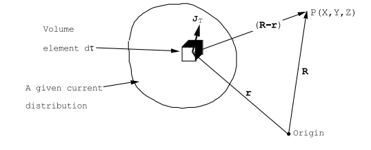
It is instructive to rewrite this equation explicitly in terms of the co-ordinates that specify the point of observation, \(\vec{\text{R}}=\text{X} \hat{\text{u}}_{x}+\text{Y} \hat{\text{u}}_{y}+\text{Z} \hat{\text{u}}_{z}\) and the coordinates that specify the position of the source element of volume \(\vec{\text{r}}=\text{x} \hat{\text{u}}_{x}+\text{y} \hat{\text{u}}_{y}+\text{z} \hat{\text{u}}_{z}\), see Figure (4.1.1):

\[\vec{\text{A}}(\text{X}, \text{Y}, \text{Z})=\frac{\mu_{0}}{4 \pi} \int \int \int_{S p a c e} d x d y d z \frac{\vec{\text{J}}_{\text{T}}(x, y, z)}{\sqrt{(\text{X}-\text{x})^{2}+(\text{Y}-\text{y})^{2}+(\text{Z}-\text{z})^{2}}}. \label{4.14} \]

The particular solution, Equation (\ref{4.14}), corresponds to the choice div(\(\vec A\)) = 0.

Derivatives of the components of \(\vec A\) with respect to the field co-ordinates (X,Y,Z) can be calculated using Equation (\ref{4.14}) by differentiating under the integral sign. For example,

\[\frac{\partial \text{A}_{\text{x}}}{\partial \text{Y}}=-\frac{\mu_{0}}{4 \pi} \int \int \int_{S p a c e} d x d y d z \frac{\left.\text{J}_{\text{T}}\right)_{x}(x, y, z)(\text{Y}-\text{y})}{\left[(\text{X}-\text{x})^{2}+(\text{Y}-\text{y})^{2}+(\text{Z}-\text{z})^{2}\right]^{3 / 2}}. \nonumber \]

Figure \(\PageIndex{2}\): A thin wire carrying a current of I Amps. The field is to be calculated at P, the point of observation.

Carrying out the differentiations term by term one can show that

\[\vec{\text{B}}(\vec{\text{R}})=\operatorname{curl}(\vec{\text{A}})=\frac{\mu_{0}}{4 \pi} \int \int \int_{S p a c e} d \tau \frac{(\vec{\text{J}} \times(\vec{\text{R}}-\vec{\text{r}}))}{|\vec{\text{R}}-\vec{\text{r}}|^{3}}, \label{4.15}\]

where d\(\tau\) is the element of volume.